Modeling Powerbus with CST
|
Geometry and setup |
Double-sided PCB:
- Size: 125 mm *100 mm *1 mm
- Top and bottom metal: PEC
- Dielectric: FR4, εr = 4.5,
loss tangent = 0.015 @ 1 GHz (Specification: Const. fit tan delta)
Model parameters:
- Frequency: 5 MHz - 2 GHz
- Steady state accuracy limit: -50 dB
Mesh
definition:
- Mesh type: Hexahedral
- Mesh density control: Lines per wavelength = 40, Others = Default
- Special mesh properties:
Refine at PEC/lossy metal edges
by factor = 6, Others = Default
- Automesh
Excitation: Discrete port
(1 V, 50 ohms)
 cst_powerbus.zip cst_powerbus.zip
|
|
Simulation result |
Simulation time: 38 mins, 43 secs
Number of mesh cells: 248864
Excitation duration: 3.563457e+000 ns
Calculation time for excitation: 152 secs
Number of calculated pulse widths: 19.9997
Simulated number of time steps: 62402
Maximum number of time steps: 62402
|
|
Decisions the user must make that affect the
accuracy of the result |
- Mesh density control: the minimum Lines per wavelength is 40.
- Special mesh properties: 6 or greater value is needed for 'Refine at PEC/lossy metal
edges by factor' to obtain higher accuracy.
|
|
Comments |
- What source do we use in this example?
In this example, we build two models to get all the results.
One model uses 'S-Parameter' port type with impedance of 50 ohms to
get the input impedance. The other model uses 'Voltage' port type with
voltage of 1.0 volts connected with a 50 ohms impedance in series to get the electric field.
- Can CST model dielectric materials with constant loss
tangent?
CST cannot model materials with constant loss tangent.
In this model, we model the dielectrics having a loss tangent of 0.015 at 1 GHz
and select the specification of
'Const. fit tan delta'.
More
information... | |
|
Screen shots
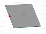
Fig. 1. Simulation model
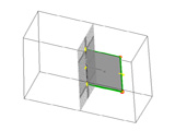
Fig. 2. Simulation meshes
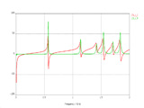
Fig. 3. Input impedance
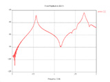
Fig. 4. Electric field at 3 m,
theta=0o, phi=0o
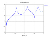
Fig. 5. Electric field at 3 m,
theta=90o, phi=0o
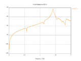
Fig. 6. Electric field at 3 m,
theta=90o, phi=90o | |
)
)
)
)
)
)