Center-Driven Dipole

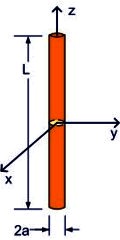
The dipole antenna is one of the simplest radiating structures. This was chosen as a canonical problem because it is relatively easy to model and analytical solutions are available. We plot the real and imaginary parts of the input impedance as a function of frequency. Codes based on the solution of surface integral equations (e.g. boundary element methods) should be able to solve this problem in a few seconds or less. Differential-equation based codes (e.g. FEM and FDTD methods) are less well-suited to this type of problem, but should still be able to produce an accurate solution in a relatively short time.

Modeling Notes:

The wire has a circular cross section with a 1-mm radius. However, equivalent results can be obtained by modeling the wire with a flat ribbon that has a 4-mm width.
The wire is 1 meter long and is modeled at frequencies from 50 - 400 MHz. In this frequency range, the length of the wire varies from 1/6th of a wavelength to 1.33 wavelengths.

Geometry	Dipole length L = 1 m Dipole radius a= 1 mm
Material	Perfect Electric Conductor (PEC) dipole in free space
Excitation	Voltage Source (1 V, 50 ohms ) or Current Source (0.02 A, 50 ohms ) Location: center of the dipole
Output	Plots of real and imaginary parts of input impedance (50 MHz - 400 MHz ) Values of input resistance and reactance at 150 MHz Frequency where Im{ Z_in }=0