Modeling a Center-Driven Dipole with EMAP
Geometry and setup |
Geometry: L= 1 m, a = 0.5 mm
Excitation: Voltage source (1 V, 50 ohms)
Mesh Setup:
- Aspect Ratio: less than 5
Frequency Setup: 50 MHz - 500 MHz, Step Size = 5 MHz
|
Simulation result |
Simulation Time: 25 mins
Number of triangles: 400
|
Decisions the user must make that affect the accuracy of the result |
- Width of ribbon: thinner better (dependent on RAM)
- Number of triangles: more better
- Aspect ratio of triangles: less than 5
|
Comments |
- How is the round wire modeled in EMAP?
The round wire is modeled as a flat ribbon PEC with vanishing thickness in EMAP.
The width of the ribbon is equal to 4 times the radius of the dipole rod.
- What kind of source is used to model this dipole in EMAP and how is it placed?
For the ribbon PEC dipole model, a voltage source is used. The amplitude of the voltage is
assigned to one of the edges in the input file of EMAP. Normally this edge is perpendicular to the axis of the dipole.
- What mesh and simulation method are used to model this dipole in EMAP?
In EMAP, all the external or surface metal is meshed as triangles. The density and aspect ratio
can be controlled with the meshing software. For the dipole model, only metal is used. Thus, only the Method
of Moments (MOM) part of EMAP is used to calculate the surface current. The code automatically
checks whether MOM and/or FEM parts are needed for the calculation.
- What is the necessary input for EMAP and what output is available from EMAP?
The geometry description file is needed for EMAP to work correctly. In the input file, the position
of the nodes, edges of triangles, edges of tetrahedrons, and their material properties must be assigned.
The input also describes the source and/or load, and whether there is an infinite ground plane.
The first result from obtained from EMAP is the surface current. For the dipole model, the current
density normal through
every edge is given. The current density times the length of the edge length gives the actual current goes
across the edge. Using the current obtained through the source edge, together with the source voltage, the
input impedance of the dipole is obtained.
If required, the far-field electrical fields can be calculated with the surface current obtained in last step.
This is accomplished with the portion of code named farcode in EMAP.
For all the results, raw data is output as a .txt file. The user can import this data into other programs
(in this case, Matlab) for post-processing.
|
|
|
Screen shots
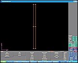
Fig. 1. Simulation model
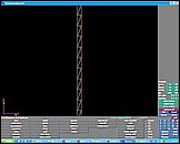
Fig. 2. Simulation meshes
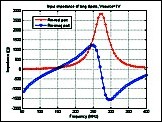
Fig. 3. Input impedance
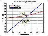
Fig. 4. Input impedance at the first resonant frequency
|
|
)
)
)
)