Can Microstripes model a dielectric material with constant loss tangent?

Modeling the Powerbus with Microstripes

Since we couldn't specify a constant loss tangent, the conductivity of the dielectric was set to 0.005. This corresponds to a loss tangent of 0.02 at 1 GHz. This resulted in more loss at low frequencies and less loss at high frequencies than specified in the statement of the problem. If we adjust the conductivity to match the loss tangent at any one frequency of interest, we can get nearly the same results at those frequencies that were obtained by codes capable of modeling constant loss tangent materials. Figures 2 - 7 show the results obtained when the conductivity was set to match a loss tangent of 0.02 at 567.646 MHz, 1.136 GHz, 1.418GHz, 1.536 GHz, 1.707 GHz and 1.828 GHz respectively. The peak impedances obtained in each case closely match results obtained using the EMAP and HFSS codes, which are shown in Figures 8 and 9.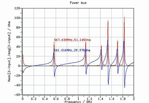

Fig. 2. Input Impedance when loss tangent is 0.02 at 567.646 MHz.

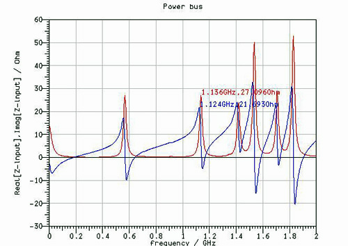
Fig. 3. Input Impedance when loss tangent is 0.02 at 1.136 GHz.

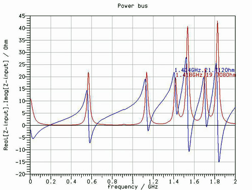
Fig. 4. Input Impedance when loss tangent is 0.02 at 1.418 GHz

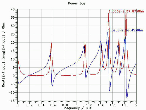
Fig. 5. Input Impedance when loss tangent is 0.02 at 1.536 GHz

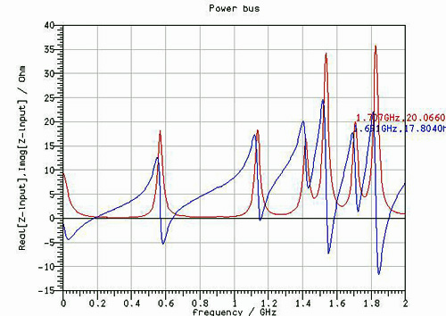
Fig. 6. Input Impedance when loss tangent is 0.02 at 1.707 GHz

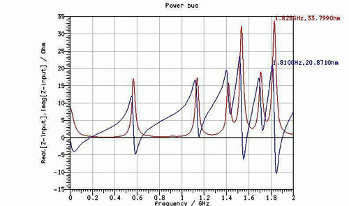
Fig. 7. Input Impedance when loss tangent is 0.02 at 1.828 GHz

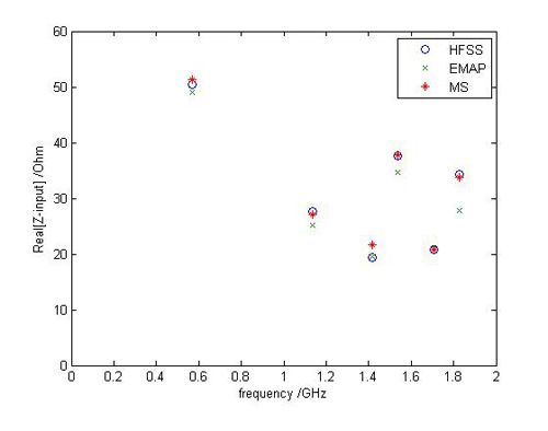
Fig. 8. Comparison of the peak values of the input impedance (real part) obtained using HFSS, EMAP, and MicroStripes

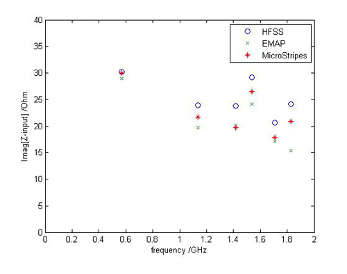
Fig. 9. Comparison of the peak values of the input impedance (image part) obtained using HFSS, EMAP, and MicroStripes