Modeling a Powerbus with IE3D
|
Geometry and setup |
Double-sided PCB:
- Size: 125 mm × 100 mm × 1 mm
- Top and bottom metal: PEC
- Dielectric: FR4, εr = 4.5,
dielectric loss tangent = 0.015
Simulation Setup:
- Meshing parameters: meshing frequency = 2 GHz, cells/wavelength = 15
- Mesh alignment is enabled: Align polygons and dielectrics
- Adaptive Intelli-Fit (AIF): disabled
- Matrix solver: default SVSa
- Frequency Parameters: 5 MHz - 2 GHz, Step Size = 5 MHz
- Excitation: Voltage source (1 V, 50 ohms)
 ie3d_powerbus.zip ie3d_powerbus.zip
|
|
Simulation result |
Simulation Time: 5111 seconds
Number of Cells/Volumes/Unknowns: 300/143/1136 |
|
Decisions the user must make that affect the
accuracy of the result |
- Define the dielectric block as a finite substrate: By default, the substrate size is infinitely large in IE3D.
In this case, the dielectric block should be defined as a finite substrate. Please refer to the comments for
details.
- Align meshing between the polygons and the finite dielectric: The meshing alignment between
the finite dielectrics and the patch is extremely critical to the simulation results.
- Define a port as a pair of positive and negative terminals: When there is no infinite ground plane, a user
needs to define a port as a pair of positive and negative terminals. Numerical error may be introduced if we
don't define a port in pair (+, -) or define a differential port (vertical localized or horizontal localized
port with self-contained + and - terminals) on a structure without an infinite ground plane.
|
|
Comments |
|
| |
Screen shots
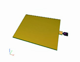
Fig. 1. Simulation model
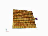
Fig. 2. Simulation meshes
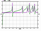
Fig. 3. Input impedance
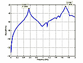
Fig. 4. Electric field at 3 m,
θ=0°, φ=0°
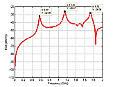
Fig. 5. Electric field at 3 m,
θ=90°, φ=0°
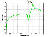
Fig. 6. Electric field at 3 m,
θ=90°,
φ=90° | |
)
)
)
)
)
)