The Boundary Element MethodBoundary Element Method (BEM) codes use the method of moments to solve an EFIE, MFIE or CFIE for electric and/or magnetic currents on the surfaces forming the interfaces between any two dissimilar materials. Most CEM modeling codes that bill themselves as simply "moment method" codes employ a boundary element method.
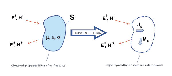
Figure 1: Principle of Equivalence. The first step in a boundary element analysis is to represent the problem geometry as a distribution of equivalent surface currents in a homogeneous medium (usually free space). As illustrated in Figure 1, the fields exterior to an object consist of fields incident on the object, fields reflected from the object and fields emanating from the object. The Equivalence Theorem [1] states that any field distribution exterior to an object can be exactly duplicated by removing the object and replacing it with a set of equivalent electric and magnetic currents on the boundary surface. Since the forms of EFIE and MFIE used by boundary element methods are only valid for current distributions in a uniform homogeneous medium, all objects in the problem space must be removed and replaced with (initially unknown) surface currents conforming to their boundaries. Equations (1) and (2) below show a common form of the EFIE and MFIE employed by boundary element method codes that model metallic objects only (i.e. there are no equivalent magnetic surface currents);
In these equations, The functions Ge and Gm in these equations relate source currents to the electric and magnetic field generated by those currents, respectively. Ge and Gm are called Green's functions [2] and they play a central role in boundary element analysis. Free-space Green's functions express the field emanating from the surface current represented by an individual basis function (e.g. the current on an individual surface patch). However, other Green's functions can be employed to express the field emanating from more complex structures that are common to a particular problem geometry. For example, a geometry consisting of metal surfaces coated with a thin dielectric may employ a special Green's function that expresses the fields emanating from the combined surfaces of the metal-dielectric and dielectric-air interfaces. This can substantially reduce the number of surface elements required to model the problem. All Green's functions are approximate expressions that are accurate for a limited range of frequencies, distances and source geometries. Many boundary element methods employ several Green's functions to model different regions of a problem or different problem environments. General purpose 3D BEM codes usually employ basis and weighting functions that are linear current distributions on a rectangular or triangular surface patch. There are generally two unknowns per patch corresponding to two orthogonal current vectors. Thin wires can be represented very efficiently with a single unknown representing the amplitude of the current distribution on each wire segment. Point matching techniques employ basis and weighting functions that are simple impulse functions often at the center of each patch or segment. Pulse matching techniques employ basis and weighting functions that have a constant value everywhere on the patch or segment. More accurate implementations employ basis and weighting functions that transition smoothly from one patch to the next. Rao-Wilton-Glisson (RWG) [3] basis functions are a popular choice for codes that employ triangular surface patch elements. Roof-top basis functions [4] are often employed by codes that use rectangular elements. Generally, CEM software employing a boundary element method excels at modeling unbounded problems, particularly when it is not necessary to model regions of great complexity in detail. Structures that can be adequately represented with a wire grid can be analyzed very effectively using boundary element methods, because these methods model wires very efficiently. Table 2 lists various strengths and weakness of BEM modeling techniques. Note that the capabilities of any particular modeling software depend strongly on the form of the integral equation solved, the choice of basis and weighting functions, the Green's function(s) employed, and the matrix solver and any optimization techniques employed. Table 2: Strengths and Weaknesses of the Boundary Element Method
Table 3 lists various CEM modeling codes that are based on a boundary element method. The codes listed and the comments in Table 3 are based on the information available to the authors as of the publication date of this report. Table 3: CEM Modeling Codes that use the Boundary Element Method
References[1] R. F. Harrington, Time Harmonic Electromagnetic Fields, New York, McGraw Hill, 1961, Ch. 3. [2] R. E. Collin, Field Theory of Guided Waves, 2nd ed., New York, IEEE Press, 1991, Ch. 2. [3] S. M. Rao, D. R. Wilton, and A. W. Glisson, "Electromagnetic scattering by surfaces of arbitrary shape," IEEE Trans. Antennas Propagat., vol. 30, pp. 409-418, May 1982. [4] D. C. Chang and J. X. Zheng, "Electromagnetic modeling of passive circuit elements in MMIC," IEEE Trans. on Microwave Theory and Tech., vol. 40, no. 9, pp. 1741-1747, Sep. 1992. |