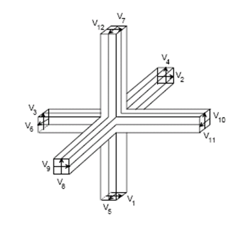
The Transmission Line Matrix Method

The Transmission Line Matrix (TLM) method, introduced by Johns [1], is similar to the FDTD method in terms of its capabilities, but its approach is unique. Like FDTD, analysis is performed in the time domain and the entire region of the analysis is gridded. Instead of interleaving E-field and H-field grids however, a single grid is established and the nodes of this grid are interconnected by virtual transmission lines. Excitations at the source nodes propagate to adjacent nodes through these transmission lines at each time step.

The symmetrical condensed node formulation introduced by Johns [2] has become the standard for three-dimensional TLM analysis. The basic structure of the symmetrical condensed node is illustrated in Figure 4. Each node is connected to its neighboring nodes by a pair of orthogonally polarized transmission lines.

Figure 4: The Symmetrical Condensed Node.

Absorbing boundaries are easily constructed in TLM meshes by terminating each boundary node transmission line with its characteristic impedance. Simons and Bridges [3, 4] derived 2D TLM absorbing boundaries, Saguet [5] proposed matched load simulation based on a Taylor series expansion technique for 2D TLM waveguide problems. Morente et al. [6] investigated TLM absorbing boundaries based on a one-way equation technique for three-dimensional problems. Chen [7] implemented absorbing and connecting boundary conditions into a 3D TLM simulation based on Higdon's absorbing conditions, a Taylor expansion algorithm, and connecting boundary conditions. Kukutsu [8] presented a super absorption boundary condition for guided waves. Eswarappa [9] and Pena [10] describe an algorithm that interfaces the three-dimensional (3D) transmission-line matrix (TLM) with an absorbing-boundary condition (ABC) based on the perfectly matched-layer (PML) approach. Shao [11] implemented a Z-transform based absorbing boundary condition.

Generally, dielectric loading is accomplished by loading the nodes with reactive stubs. These stubs are usually half the length of the mesh spacing and have a characteristic impedance appropriate for the amount of loading desired. Lossy media can be modeled by introducing loss into the transmission line equations or by loading the nodes with lossy stubs. De Menenes [12-14] presented the modeling of a nonlinear Lorentz dielectric and a frequency independent dielectric with a Kerr nonlinearity. Hein [15, 16] developed the TLM model for propagation in both magnetized plasma and ferrite. Paul [17-19] designed TLM algorithms for one-dimensional (1D) and three-dimensional (3D) models involving linear frequency-dependent isotropic dielectric media, anisotropic materials, and frequency dependent nonlinear dielectric materials.

The strengths of the TLM method are similar to those of the FDTD method. Complex, nonlinear materials are readily modeled. Impulse responses and the time-domain behavior of systems are determined explicitly. And, like FDTD, this technique is suitable for implementation on massively parallel machines.

Both the TLM and FDTD techniques are powerful and widely used. For many types of EM problems they represent the only practical methods of analysis. Deciding whether to utilize a TLM or FDTD technique is often based on personal preference. Many engineers find the transmission line analogies of the TLM method to be more intuitive and easier to work with. On the other hand, others prefer the FDTD method due to its simple, direct approach to the solution of Maxwell's field equations. For modeling propagation in complex materials, TLM may offer a more straightforward solution than FDTD. Also, the TLM method generally does a better job of modeling complex boundary geometries, because both E and H are calculated at every boundary node. However, TLM methods require more computer memory per node than FDTD.

References

[1] P. B. Johns and R. L. Beurle, "Numerical solution of 2-dimensional scattering problems using a transmission-line matrix," Proc. Inst. Elec. Eng., vol. 118, no. 9, pp. 1203-1208, 1971.

[2] P.B. Johns, "A symmetrical condensed node for the TLM method," IEEE Trans. on Microwave Theory and Tech., vol. 35, no. 4, pp. 370-377, 1987.

[3] N. R. S. Simons and E. Bridges, "Method for modelling free space boundaries in TLM simulations," Electronics Letters, vol. 26, no. 7. pp. 453-155, Mar., 1990.

[4] N. R. S. Simons and E. Bridges, "Application of the TLM method to two-dimensional scattering problems." Int. J. Num. Modelling: Electron. Network Devices, Fields, vol. 5. pp. 93-119, 1992.

[5] P. Saguet, "TLM method for the three dimensional analysis of microwave and mm-wave structures." Paper presented at Int. Workshop of the German IEEE M7T/AP Chapter on CAD Oriented Numerical Techniques for the Analysis of Microwave and MM-Wave Transmission-Line Discontinuities and Junctions, Stuttgart, Germany, Sept. 13, 1991.

[6] J. A. Morente, J. A. Porte, and M. Khalladi, "Absorbing boundary conditions for the TLM method," IEEE Trans. on Microwave Theory and Tech., vol. 40, no. 11, pp. 2095-2099, 1992.

[7] Z. Chen, M. M. Ney, and W. J. R. Hoefer, "Absorbing and connecting boundary conditions for the TLM method," IEEE Trans. on Microwave Theory and Tech., vol. 41, pp. 2016-2024, Nov. 1993.

[8] N. Kukutsu and R. Konno, "Super absorption boundary condition for guided waves in the 3-D TLM simulation," IEEE Microwave Guided Wave Lett., vol. 5, pp. 299-301, Sep. 1995.

[9] C. Eswarappa, and W.J.R. Hoefer, "Implementation of Berenger absorbing boundary conditions in TLM by interfacing FDTD perfectly matched layers," Electronics Letters, vol. 31, no. 15, pp. 1264-1266, 1995.

[10] N. Pena, and M. M. Ney, "Absorbing-boundary conditions using perfectly matched-layer (PML) technique for three-dimensional TLM simulations," IEEE Trans. on Microwave Theory and Tech., vol. 45, no. 10 pp. 1749-1755, 1997.

[11] Z. Shao, W. Hong, and H. Wu, "A Z-transform-based absorbing boundary conditions for 3-D TLM-SCN method," IEEE Trans. on Microwave Theory and Tech., vol. 50, no. 1, pp. 222-225, 2002.

[12] L. de Menezes and W. J. R. Hoefer, "Modeling nonlinear dispersive media in 2D TLM," Proc. 24th European Microwave Conf., pp. 1739-1744, Sept. 1994.

[13] L. de Menezes and W. J. R. Hoefer, "Modeling frequency dependent dielectrics in TLM," 1994 IEEE APS Symp. and URSI Meet. Dig., Seattle, WA, pp. 1140-1143, Jun. 1994.

[14] L. de Menezes and W. J. R. Hoefer, "Modeling of general constitutive relationships using SCN TLM," IEEE Trans. on Microwave Theory and Tech., vol. 44, pp. 854-861, June 1996.

[15] S. Hein, "Synthesis of TLM algorithms in the propagator integral framework," 2nd Int. Workshop Transmission-Line Matrix (TLM) Modeling Theory Applicat., Tech. Univ., Munich, Germany, pp. 1-11, Oct. 1997.

[16] S. Hein, "TLM numerical solution of Bloch's equations for magnetized gyrotropic media," Appl. Math. Modeling, vol. 21, pp. 221-229, Apr. 1997.

[17] J. Paul, C. Christopoulos, and D. W. P. Thomas, "Generalized material models in TLM -part 1: Materials with frequency-dependent properties," IEEE Trans. Antennas Propagat., vol. 47, pp. 1528-1534, Oct. 1999.

[18] J. Paul, C. Christopoulos, and D. W. P. Thomas, "Generalized material models in TLM -part 2: Materials with anisotropic properties," IEEE Trans. Antennas Propagat., vol. 47, pp. 1535-1542, Oct. 1999.

[19] J. Paul, C. Christopoulos, and D. W. P. Thomas, "Generalized material models in TLM -part 3: Materials with nonlinear properties," IEEE Trans. Antennas Propagat., vol. 50, pp. 997-1004, Jul. 2002.