Laguerre formula

Absolute points have a surprising but important application: they can be used to determine the angle between two lines. To see how this works, let us assume that we have two lines $\ensuremath{{\bf u}} _1$ and $\ensuremath{{\bf u}} _2$ which intersect the ideal line at two points, say $\ensuremath{{\bf p}} _1$and $\ensuremath{{\bf p}} _2$. Then, the cross ratio between these two points and the two absolute points $\ensuremath{{\bf i}}$ and $\ensuremath{{\bf j}}$ yields the directed angle $\theta$ from the second line to the first:

$$\theta = \frac{1}{2i}\log{Cr(\ensuremath{{\bf p}} _1, \ensure... ...{{\bf p}} _2 ; \ensuremath{{\bf i}} , \ensuremath{{\bf j}} )},$$

which is known as the Laguerre formula.

To gain some intuition on why this formula is true, let us consider a simple example. Suppose we have two lines

$$\begin{eqnarray*}a_1 x - y & = & 0 \\ a_2 x - y & = & 0 \end{eqnarray*}$$

in the affine plane. It is clear that these two lines can be represented as two vectors $\ensuremath{{\bf v}_{1}} = [1, a_1]^T$and $\ensuremath{{\bf v}_{2}} = [1, a_2]^T$ in the Euclidean plane. The directed angle between the two lines is the directed angle between the two vectors and is given by:

$$\tan \theta = \frac {\ensuremath{{\bf v}_{2}}\times \ensurema... ...}}\cdot \ensuremath{{\bf v}_{2}} } = \frac{a_1-a_2}{1+a_1a_2}.$$

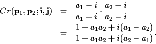
Now in the projective plane these lines are represented as [a₁, -1, 0]^T and [a₂, -1, 0]^T, which are found by mapping points [x,y]^T in the affine plane to points [x,y,1]^T in the projective plane. The ideal line passing through $\ensuremath{{\bf i}} = [1,i,0]^T$ and $\ensuremath{{\bf j}} = [1,-i,0]^T$ is given by $\ensuremath{{\bf i}}\times \ensuremath{{\bf j}} = [0, 0, 1]^T$. The two points of intersection between this line and the two original lines are given by [1, a₁, 0]^T and [1, a₂, 0]^T. The cross ratio of the four points is then given by:

$$\begin{eqnarray*}Cr(\ensuremath{{\bf p}} _1, \ensuremath{{\bf p}} _2 ; \ensurema... ..._2-i} \\ & = & \frac{1+a_1a_2+i(a_1-a_2)}{1+a_1a_2+i(a_2-a_1)}. \end{eqnarray*}$$

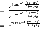
Converting the complex numbers from rectangular to polar coordinates yields:

$$\begin{eqnarray*}& = & \frac{e^{i\tan^{-1}{\frac{(a_1-a_2)}{1+a_1a_2}}}} {e^{i\... ...+a_1a_2}}}} \\ & = & e^{2i\tan^{-1}\frac{(a_1-a_2)}{1+a_1a_2}}, \end{eqnarray*}$$

from which it follows that

$$\frac{1}{2i}\log{Cr(\ensuremath{{\bf p}} _1, \ensuremath{{\bf... ...}} }{\ensuremath{{\bf v}_{1}}\cdot \ensuremath{{\bf v}_{2}} },$$

which is the desired result.