Modeling Powerbus and Cable with CST
|
Geometry and setup |
Double-sided PCB:
- Size: 125 mm *100 mm *1 mm
- Top and bottom metal: PEC
- Dielectric: FR4, εr = 4.5,
loss tangent = 0.015 @ 1 GHz (Specification: Const. fit tan delta)
Cable (flat ribbon):
- Length: 1000 mm
- Width: 8 mm
- Material: PEC
Model parameters:
- Frequency: 5 MHz - 2 GHz
- Steady state accuracy limit: -40 dB
Mesh
definition:
- Mesh type: Hexahedral
- Mesh density control: Lines per wavelength = 40, Others = Default
- Special mesh properties:
Refine at PEC/lossy metal edges
by factor = 6, Others = Default
- Automesh
Excitation: Discrete port
(1 V, 50 ohms)
 cst_powerbus_cable.zip cst_powerbus_cable.zip
|
|
Simulation result |
Simulation time: 10 hrs, 19 mins, 24 secs
Number of mesh cells: 8012970
Excitation duration: 3.563457e+000 ns
Calculation time for excitation: 4717 secs
Number of calculated pulse widths: 17.0145
Simulated number of time steps: 53789
Maximum number of time steps: 63227
|
|
Decisions the user must make that affect the
accuracy of the result |
- Mesh density control: the minimum Lines per wavelength is 40.
- Special mesh properties: 6 or greater value is needed for 'Refine at PEC/lossy metal
edges by factor' to obtain higher accuracy.
- Boundary: 'Automatic minimum distance to structure' is set to 2th part of wave.
- Low frequency: a separate model focused on low frequencies is created to replace the low frequency part (5 MHz - 300 MHz).
|
|
Comments |
- What source do we use in this example?
In this example, we use 'Voltage' port type with
voltage of 1.0 volts connected with a 50 ohms impedance in series to get the electric field.
- Can CST model dielectric materials with constant loss
tangent?
CST cannot model materials with constant loss tangent.
In this model, we model the dielectrics having a loss tangent of 0.015 at 1 GHz
and select the specification of
'Const. fit tan delta'. See the comment in the second example to get more
information...
- How is the cable modeled?
A flat PEC ribbon instead of round cable is used to model the cable.
The width of the cable is 8 mm (4 times the radius of the cable).
This substitution will decrease the simulation time without sacrificing accuracy.
more
information...
- How to get the accurate results at low frequencies?
At low frequencies, a large boundary is needed. Thus a separate model focused on low frequencies is created to replace the low frequency part (5 MHz - 300 MHz). In this sub model, 'Automatic minimum distance to structure' is set to 2th part of wave at center frequency between 5 MHz to 300 MHz. This means the boundary is expanded compared to that at high frequency range. Correspondingly, the finer mesh is needed to make the model calculable. 'Lines per wavelength' is set to 50; 'Refine at PEC/lossy metal edges by factor' is set to 6, 'Mesh line ratio limit' is set to 80; 'Steady state accuracy limit' is set to -50 dB. It took another 3 hours to solve this sub model for low frequency part.
| |
|
Screen shots
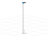
Fig. 1. Simulation model
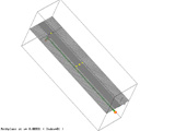
Fig. 2. Simulation mesh
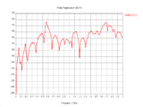
Fig. 3. Electric field at 10 m,
theta=0o, phi=0o
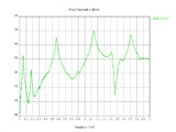
Fig. 4. Electric field at 10 m,
theta=90o, phi=0o
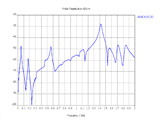
Fig. 5. Electric field at 10 m,
theta=90o, phi=90o | |
)
)
)
)
)