Modeling a Center-driven Dipole with HFSS (version 11.1.3)
|
Geometry and setup |
Geometry: L= 1 m,
a = 0.5 mm
Excitation: Lumped Port, 50
ohms
Mesh operation: Maximum length of elements=50 mm
Analysis Setup:
- Solution Frequency: 300 MHz
- Maximum Number of Passes: 50
- Maximum ΔS: 0.01
- Do Lambda Refinement: 0.5
- Maximum Refinement Passes: 20%
Sweep:
- Sweep type: Interpolate
- Frequency: 50 MHz - 400 MHz, Step Size = 5
MHz
 hfss_dipole.zip hfss_dipole.zip
|
|
Simulation result |
Simulation Time: 3
mins 47 secs
Number of passes completed: 6
Number of tetrahedra: 14073
|
|
Decisions the user must make that affect the
accuracy of the result |
- Location of absorbing boundary: λ/4
(at 300 MHz) away from the object
- Source type: use lumped port
- Maximum ΔS: default value = 0.02, this model=0.01
- Do lambda refinement: default value=0.33, this model=0.5
- Mesh operation: restrict the maximum length of elements
- Dipole material: perfect conductor
|
|
Comments |
- What if we model the wire as a
flat ribbon?
We can substitute a 2-mm wide flat ribbon
for the 0.5-mm round wire. The results are nearly the same.
More information
...
- Where was the absorbing boundary
located?
In HFSS, radiation boundaries are used to simulate
open problems that allow waves to radiate to the far field. The
accuracy of the radiation approximation depends on the distance
between the boundary and the radiation source. The radiation
surface must be located at least one-quarter wavelength from the
radiating source. It should usually also be at a distance greater
than the maximum dimension of the source.
For this
simulation, the solution frequency is 300 MHz (λ = 1 m). The
radiation boundary is defined on a cylinder whose radius is 500 mm
and height is 2000 mm. | |
|
Screen shots
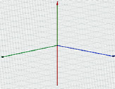
Fig. 1. Simulation model
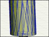
Fig. 2. Simulation meshes
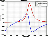 </> </>
Fig. 3. Input impedance
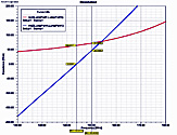
Fig. 4. Input impedance at the first
resonant frequency | |
)
)
)
)