Modeling a Center-driven Dipole with IE3D
|
Geometry and setup |
Geometry: L= 1 m,
a = 0.5 mm
De-embedded scheme: Advanced extension
Wire model: Tube (number of sides = 6)
Simulation Setup:
- Meshing Parameters: 4GHz. 100 Cells/Wavelength
- Scheme: Classical, No FASTA
- Matrix Solver: Adaptive Symemtric Solver
- Adaptive Intelli-Fit: Enabled
- Frequency Parameters: 5 MHz - 400 MHz, step size = 5 MHz
Sweep:
 ie3d_dipole.zip
|
|
Simulation result |
Simulation Time: 61 seconds
Number of cells: 912
Number of unknowns: 1812
Input impedance at 150 MHz: 83.2+j41.2 Ohms
First resonant frequency: 144 MHz
|
|
Decisions the user must make that affect the
accuracy of the result |
- Meshing frequency and meshing cell size: Higher mesh densities or cells per wavelength generally yields more accurate results. In this example, we set the meshing frequency to 400 MHz and cells/wavelength
to 100.
- De-embedding scheme: The Advanced Extension scheme is normally the best considering the applicable frequency
range and stability.
- Adaptive Intelli-Fit (AIF): A scheme allowing users to get the frequency response at many frequency
points with guaranteed accuracy by simulating just a few frequency points. This can reduce the simulation
time significantly. Enable AIF and use the default settings.
|
|
Comments |
- Other ways to model the dipole antenna
There are few different ways to model the dipole antenna depending upon the accuracy required
More information
...
| |
|
Screen shots
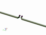
Fig. 1. Simulation model
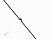
Fig. 2. Simulation meshes
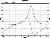 </> </>
Fig. 3. Input impedance
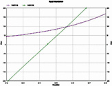
Fig. 4. Input impedance at the first
resonant frequency | |
)
)
)
)