Concentration polarization over reverse osmosis membranes with engineered surface features

Zuo Zhou , Bowen Ling , Ilenia Battiato , Scott M. Husson, David A. Ladner

Published in the Journal of Membrane Science

Citation: Zhou, Z.; Ling, B.; Battiato, I.; Husson, S.M.; Ladner, D.A. “Concentration polarization over reverse osmosis membranes with engineered surface features.” Journal of Membrane Science 2021, 617, 118199.

https://doi.org/10.1016/j.memsci.2020.118199

Abstract

Creating membranes with engineered surface features has been shown to reduce membrane fouling and increase flux. Surface feature patterns can be created by several means, such as thermal embossing with hard stamps, template-based micromolding, and printing. It has been proposed that the patterns create enhanced mixing and irregular fluid flow that increases mass transfer of solutes away from the membrane. The main objective of this paper is to explore whether enhanced mixing and improved mass transfer actually do take place for reverse osmosis (RO) membranes operated in laminar flow conditions typical of full-scale applications. We analyzed velocity, concentration, shear stress, and concentration polarization (CP) profiles for flat, nanopatterned, and micropatterned membranes using computational fluid dynamics. Our methods coupled the calculation of fluid flow with solute mass transport, rather than imposing a flux, as has often been done in other studies. A correlation between Sherwood number and mass-transfer coefficient for flat membranes was utilized to help characterize the hydrodynamic conditions. These results were in good agreement with the numerical simulations, providing support for the modeling results. Models with flat, several line and groove patterns, rectangular and circular pillars, and pyramids were explored. Feature sizes ranged from zero (flat) to 512 μm. The ratio of feature length, between-feature distance, and feature height was 1:1:0.5. Results indicate that patterns greatly affected velocity, shear stress, and concentration profiles. Lower shear stress was observed in the valleys between the pattern features, corresponding to the higher concentration region. Some vortices were generated in the valleys, but these were low-velocity flow features. For all of the patterned membranes CP was between 1% and 64% higher than the corresponding flat membrane. It was found that pattern roughness correlated with boundary layer thickness and thus the patterns with higher roughness caused lower mass transfer of solute away from the surface. Rather than enhancing mixing to redistribute solute, the patterns accumulated solute in valleys and behind surface features. Despite the elevated CP, the nominal permeate flux increased by as much as 40% in patterned membranes due to higher surface area compared to flat membranes. The advantageous results seen in other studies where patterns have helped increase flux may be caused by the additional surface area that patterns provide.

1. Introduction

Surface structure has been a topic of interest in membrane science since the early days of membrane development. Reverse osmosis (RO) membrane roughness was identified as an adverse feature that leads to increased fouling [[1], [2], [3]]. Foulants preferentially accumulated in the valleys and caused flux decline due to “valley clogging” [1]. A recent example of those lauding the effects of flat (non-rough) membranes is Chowdhurry et al. [4], where a new technology was designed to make polyamide membranes smoother to yield better performance in water desalination.

Interestingly, another effort has been underway in the field to increase surface roughness by patterning membranes in controlled ways for fouling reduction. These patterned membranes have been studied in the past few years and results show that they are an effective way to reduce fouling and improve membrane performance [[5], [6], [7], [8], [9], [10], [11]]. Flat membranes have often been described as the lowest-fouling geometry, but a growing body of work is showing that adding ordered roughness via patterns may also be effective.

A key to teasing out whether flat or patterned membranes are optimal for fouling control lies in understanding the mechanisms. A few different mechanisms are hypothesized to be instrumental in the patterns’ beneficial effects. Some papers have stated that turbulence at the apex of the pattern surface led to reduced deposition of microbial cells [5,7]. In a similar vein, other papers discuss high shear stress on the upper region of the patterns that decreases the attachment of foulants or helps re-entrain them after deposition [6,8,11]. Some claim that introduction of ordered roughness can disrupt the hydrodynamic boundary layer during flow over the membrane [9].

Our goal is to investigate the mechanisms that might make patterns beneficial in RO systems. In many of the published papers the hypotheses about foulant mitigation are related to hydrodynamics. One important contribution is from Maruf et al. [12] who studied concentration polarization (CP) on a thin-film composite (TFC) nanofiltration membrane experimentally and discovered some benefits to the patterning for improving flux and reducing scaling. This, along with the previous studies, supports the hypothesis that patterns help create mixing and improve the mass transfer of foulants away from the membrane. Often mixing is shown through vortices observed as circular flow streamlines in modeling results. Vortex formation and mixing of sufficient magnitude should also reduce CP and thus reduce the driving force needed for water permeation. CP, caused by rejection of salt ions on the membrane surface, has been widely studied in RO systems [[13], [14], [15]]. It is influenced by salt properties, membrane properties, and hydrodynamics [16,17]. It can be an important indicator of flux decline, and is a phenomenon that is related to the occurrence of fouling [[18], [19], [20]]. Studying CP can help us understand the ways in which hydrodynamics are affected by patterns.

The details of water flow in membrane channels – the hydrodynamics – are difficult to measure experimentally in the lab; mathematical models can help in this regard. Many studies have focused on analytical models to predict CP, in which the classic film theory provides an estimate of the degree of CP based on the flux and mass transport [21]. Numerical models also have been developed to combine computational fluid dynamics (CFD) and solute mass transport. Navier-Stokes, continuity, and convective-diffusion equations are coupled to solve for the fluid flow velocities in the channel above the membrane and the salt concentrations that define the CP layer and affect the water flux [13,22].

A critical piece to the numerical modeling accuracy is to use fully coupled flow and solute transport equations [13]. In one modeling approach, investigators simplified governing equations and assumed that the permeation velocity does not depend on axial position and therefore remains constant along the length of the membrane channel [23]. This decoupling of flux and solute concentration can decrease the accuracy of the models since permeate flux is affected by osmotic pressure that increases down the channel. Another group used analytical models to theoretically predict permeation flux, and used numerical simulation to predict flow and mass transfer [24]. That approach is better than assuming constant flux, but is still not a complete coupling. Xie et al. [25] studied CP in spacer filled channels by fully coupling flow and mass transport equations. They predicted CP mitigation that was consistent with experimental results. In our models, flow and mass transport equations are likewise combined to solve for mass transfer. Osmotic pressure is linearly related to salt concentration, and flux is calculated by taking into account both the hydraulic and osmotic pressures.

The approach of this study was to investigate the hydrodynamics in the channels above membranes that have various-shaped patterns covering a large size range. Literature was reviewed to determine what pattern sizes would be relevant. RO surface roughness ranges from 40 nm to 100 nm [1,26]. Lee et al. [8] designed prism patterns that were 400 μm wide and 200 μm tall. Jang et al. [27] studied both nanometer-and micrometer-scale patterns. Won et al. [7] investigated prism patterns ranging from 25 μm to 400 μm. For this study we wanted to cover a size range that would encompass all of the literature numbers, then go above and below that range. Some of the pattern sizes used here are larger than previously fabricated, but allow us to explore the limits of hydrodynamic effects. For each size we built eight geometries that cover elementary shapes including lines and grooves, pillars, and pyramids. A Sherwood correlation was compared to the data for the flat membrane and confirmed that our multi-scale models were behaving rationally compared to experiments. Mass-transfer coefficients were interpreted based on flow and concentration regimes and were used to calculate the parameters of the Sherwood correlation. A relationship between theoretical boundary layer thickness and membrane roughness was revealed. This paper provides a detailed discussion of hydrodynamic effects of patterns, including CP, shear stress, velocity streamlines, and permeate flux.

2. Materials and methods

2.1. Geometries studied

Multiple models of RO membranes patterned with varied geometries were built for analysis. The geometries include flat, several line and groove patterns, rectangular and circular pillars, and pyramids (Fig. 1). These shapes covered several elementary geometries and allowed an investigation of the hydrodynamic effects of regularly ordered surface features. Most models were created with SolidWorks and imported into COMSOL Multiphysics 5.3 using the COMSOL CAD import tool.

Fig. 1. Patterns studied include (a) flat, (b) line and groove [LG] rectangle, (c) LG trapezoid, (d) LG triangle, (e) LG circle, (f) rectangular pillars, (g) pyramids, and (h) circular pillars.

Fig. 2 shows a conceptual model for how fluid flow was simulated. To be consistent with an ongoing project in our lab, we used a feed (inlet) velocity (u_in) with a 1 m entrance length to achieve a fully developed laminar flow regime at the entrance, a feed solute concentration (c_b) of 0.025 M, and a diffusion coefficient of 10−9 m²/s at the temperature of 20 °C. The feed concentration and diffusion coefficients were chosen to fall within a range of typical values that might be found for salt-rejecting membrane systems such as brackish water desalination or softening. We chose to hold these variables constant as we studied different pattern types and sizes. Reynolds number is around 300 under all circumstances.

Fig. 2. Conceptual model for the membrane simulations. The membrane is at the bottom (pink color). The block represents the water- and solute-filled space above the RO membrane. Boundary conditions are listed in Table 1. At wall a-b-c-d water is moving parallel to the membrane surface with a velocity adjusted based on Equation (2). Wall a-b-f-e and d-c-g-h are periodic boundaries. The average inlet velocity at wall a-d-h-e is set according to the model size, also using Equation (2). Inlet concentration is 0.025 M. The pressure at the concentrate boundary is 2800 kPa. (For interpretation of the references to color in this figure legend, the reader is referred to the Web version of this article.)

Periodic boundaries were set up on both sides parallel to the flow direction (planes a-b-e-f and d-c-g-h in Fig. 2) to avoid edge effects caused by no-slip walls; this boundary condition creates a model with infinite width. At the concentrate (outlet) side, the pressure was set at 2800 kPa (400 psi), which (like the feed concentration and diffusion coefficient) is within a range of typical values for salt-rejecting membrane processes. Viscous stress and diffusive flux at the outlet were assumed to be negligible. The boundary on the top (a-b-c-d in Fig. 2) was a moving wall (see Table 1).

Table 1. Boundary conditions for membrane channel simulations. Boundary designations correspond to Fig. 2. Conditions are listed using Cartesian coordinates; for example, (0,0,u_m) designates zero flow (no slip) in the x and y directions, and a flow of um in the z direction.

The flux normal to the wall at the membrane (um) was calculated with Equation (1). The flux was set as a boundary condition at the membrane wall:

—- eq(1)

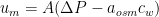
The membrane water permeability (A) was 5.24 × 10⁻¹² m/(s·Pa), the osmotic coefficient (a_osm) was 4872 Pa/(mol/m³), and the salt concentration at the membrane wall (c_W) was calculated during the simulation. The transmembrane applied pressure (ΔP) was calculated by subtracting the permeate pressure from the applied pressure calculated next to the membrane; permeate pressure was zero, so ΔP was equal to the applied pressure.

In actual RO systems, water flow is bounded by membranes above and below each flow channel. The size of the flow channel depends on the thickness of the feed spacer, typically on the order of 1 mm. This means that if a pattern is large enough (about a fourth of 1 mm or larger), the flow around the pattern would be affected not only by the pattern but also by the opposite wall bounding the flow. In designing this study, we initially used feed channels of a realistic (~1 mm) size, but noticed that the opposite-wall effects became more influential than the pattern effects as pattern size grew. To alleviate this problem, we based our simulations on channels that were 16 mm tall. We saw that this was far enough from the membrane to avoid influencing the flow patterns and CP near the membrane surface.

Another challenge in this study was its multi-scale nature; we wanted to simulate a wide range of pattern sizes to fully explore the effects of size on flow behavior. The difficulty was that if we kept the simulation size the same for all patterns, we would need a large simulation space to accommodate the large patterns, and would need extremely dense finite elements when using that large simulation space with small patterns. Instead these models simulate only a portion of the flow channel above the membrane surface; we scaled the size of the simulation box with the size of the pattern features. This approach required changing the way the inlet velocity was handled, since we expected a laminar-flow velocity profile in the channel. We applied a moving wall at plane a-b-c-d in Fig. 2, the side opposite the membrane. The average velocity uave was calculated with Equation (2), and umax is the maximum velocity when H = Hc in Fig. 3.

—- eq(2)

Fig. 3. Velocity adjustment based on planar Poiseuille flow. The total channel height 2H is assumed to be 16 mm with an average velocity u_ave = 0.1 m/s. Based on each model height H, u(H) is calculated through Equation (2), which is applied on the top wall. A new average velocity u_ave is integrated through Equation (2) and is applied at the inlet velocity.

Each model included four rows of features, making the total simulated length eight times as long as the feature length (Fig. 4). Flat membranes with the same total projected length were simulated as the control group. In this paper we refer to each model by its pattern shape and pattern size; for example, a line and groove model with a rectangular profile and a 512 μm feature length is called LG rectangle 512. The corresponding flat membrane with the same simulation block size is called Flat 512.

Each model included four rows of features, making the total simulated length eight times as long as the feature length (Fig. 4). Flat membranes with the same total projected length were simulated as the control group. In this paper we refer to each model by its pattern shape and pattern size; for example, a line and groove model with a rectangular profile and a 512 μm feature length is called LG rectangle 512. The corresponding flat membrane with the same simulation block size is called Flat 512.

Table 2 shows pattern feature sizes. Pattern lengths range from 125 nm to 512 μm, with each subsequent model being four times the length of the previous. With eight pattern styles (including flat) and seven sizes, there were 56 models in all. The feature length (l) was the same as the between-feature distance (d), while the height (h) of the features was equal to half of the length; we denote this geometric ratio as l:d:h = 1:1:0.5 (see Table 2 for details). Some initial simulations covered different ratios of feature length to between-feature distance, from 0.5 to 2, but those results did not seem to give useful insight; decreasing the ratio only made the patterns behave more like flat membranes. To keep the scope of our study reasonable, we proceeded with only one ratio of feature length to between-feature distance. This is similar to patterns described in previous work [9,12]. Due to convergence issues that result in extremely high values (singularities) around sharp edges, edges were curved by adding fillets with a radius that was one fifth of the height.

2.2. Mesh generation

The CFD models used in this work consisted of a mesh of tetrahedral finite elements that filled the space above the membrane. At and near the membrane boundary layer the meshes were much finer to characterize the steep gradient of salt concentration changes near the surface. A mesh sensitivity study was performed to determine the influence of mesh density on the results. With increasing mesh density there was a change in CP and flux values; however, the values stabilized as the density increased (Fig. S1). For example, with 512 μm-long line and groove (LG) triangular patterns, 492,078 mesh elements resulted in CP that was only 5% higher than when 350,097 mesh elements were used. Table S1 shows the mesh element numbers of all the simulations. The lowest mesh element number was 440,000 and highest was over 800,000. Mesh sensitivity tests were conducted for each model, making sure the results were independent from the mesh element numbers.

2.3. Governing equations

Fluid flow and transport of solute were described by Equations (3)–(5)

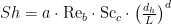
Fig. 5. CP factor results for five flat-membrane models of various sizes. The fitted curve was produced using Equations (6), (7), (8) with a = 1.85 and b = c = d = 0.275.

Here a, b, c, and d are parameters in the Sherwood correlation, d_h is hydraulic diameter, L is channel length, k is the mass-transfer coefficient, Sh is the Sherwood number, D is the diffusion coefficient, c_m is the solute concentration at the membrane surface, c_b is the bulk solute concentration, and J is water flux through the membrane. The CP factor is defined as the ratio of salt concentration at the membrane surface to bulk concentration (c_m/c_b) as shown in Equation (8). Because the model sizes change and thus a calculated bulk concentration could also change, we set c_b equal to the feed concentration (c_f) when calculating the CP factor.

The a parameter value that resulted in the best fit to the data set was a = 1.85. The b, c, and d parameters were all 0.275. These parameter values fall within the typical expected ranges for similar processes [28,29]. This gives us confidence that our Sherwood correlation equation was valid and that the models were behaving similarly to the experiments that were used to create the Sherwood correlations in the literature. More importantly, the models for systems with different membrane sizes gave data that converged onto one master curve, lending credibility to our methods for multi-scale modeling (Fig. S2 in Supporting Information is a plot without velocity adjustment for comparison.).

3.2. Concentration and shear stress

The solute concentration profiles for flat-membrane models showed a low concentration at the entrance with a gradual increase toward the downstream end, as would be expected (Fig. 6). CP was manifest with a high concentration near the membrane surface and a decrease toward the bulk solution. For patterned membranes, a high concentration accumulated in the valleys and a much lower concentration was seen at the apex of the features.

Fig. 6. Concentration profiles along the membrane surface for flat and the seven patterns of interest. Shown here are results from the 512 μm feature size models. Results from other sizes looked similar, though the maximum concentrations were lower. Cut plane results are shown on the right. For the patterns that are not heterogeneous in the direction that is perpendicular to the page, two cut planes were chosen: one is between two features and one cuts through the middle of a feature.

Fig. 7 compares the concentration profile along the longitudinal axes of the LG rectangle, LG trapezoid, LG triangle, and Flat 512 models. The flat-membrane results show a classic CP boundary layer development, with concentration gradually increasing from entrance to exit. In the LG trapezoid results there was a periodically fluctuating concentration profile. At the elevated portions of the pattern (the “peaks,” or “plateaus” in this case) the concentration is lower than would be present in the flat-membrane case, giving some credence to the idea that patterns can help lower CP. But in the valleys the concentration is much higher than the flat-membrane case; the net result for the entire membrane is that the LG pattern caused an increase in CP.

Fig. 7. Concentration profile along the membrane surface for (1a, 1b) LG Rectangle 512, (2a, 2b) LG Trapezoid 512, and (3a, 3b) LG Triangle 512. Concentration profiles for (1c, 2c, 3c) Flat 512 are also shown. All geometries are aligned for parallel comparison.

The analysis performed above to compare the LG trapezoid with its flat-membrane analog was repeated for all 40 pattern models. CP factors were calculated and normalized to the analogous flat-membrane CP factor (Fig. 8). All of the data points fall above the flat-membrane dotted line, indicating that all patterns (and all sizes) increased CP. We tested different salt concentrations, different diffusion coefficients, and crossflow velocities, and the overall conclusion remained the same: CP was always elevated in patterned membranes compared to flat ones. So here we are only reporting one salt concentration (25 mol/m³), one diffusion coefficient (10⁻⁹ m²/s), and one crossflow velocity (0.1 m/s).

Fig. 8. CP results normalized to flat membranes with the same block size. All seven sizes are presented (0.125, 0.5, 2, 8, 32, 128, and 512 μm). Feed concentration was 25 mol/m³ and the diffusion coefficient was 10⁻⁹ m²/s. Crossflow velocity was scaled as described in Fig. 3 to model a 0.1 m/s flow channel.

Shear stress profiles showed the opposite trend from the concentration profiles, with the highest shear in the apex of the patterns and the lowest in the valleys (Fig. 9). Values decreased along the length of the channel with each peak value being smaller (shown with red color that fades to orange-yellow; this is most obvious in the LG rectangle pattern, Fig. 9b). These results are consistent with the idea that higher shear stress reduces CP [25,30].

Fig. 9. Shear stress profiles along the membrane surface for flat and the seven patterns of interest. Letters indicate the same geometries designated in Fig. 1, Fig. 6. Shown here are results from the 512 μm feature size models. Results from other sizes looked similar, though the shear stress values differed.

3.3. Velocity profile and streamlines

Velocity was studied to investigate the mixing condition in the system. In general, the velocity profile fits the expected distribution for planar Poiseuille flow between two parallel plates, with lower values near the no-slip boundary and higher values increasing toward the center of the geometry [31]. Fig. 10 shows the velocity profile near the surface of the Flat and LG rectangle 512 membranes.

Fig. 10. Velocity profile near the membrane surface for (a) Flat 512 and (b) LG rectangle 512. The simulation space in the graph is 800 μm above the membrane surface.

Some vortices were observed in the valleys between the features (Fig. 11). These vortices act like lid-driven cavities, which is a benchmark problem in CFD [32]. Flow symmetries were distorted and stream directions were changed; however, the velocities for these vortices were low. Others have discussed vortex formation being helpful in the removal of foulants in patterned membranes [8,12]. Here, though we also observed vortices, they did not promote enough mass transfer of salt away from the membrane surface to decrease CP.

Fig. 11. Streamline profile for LG rectangle 512. The color indicates the velocity. Vortices are seen in between features with low velocities (shown in blue color). (For interpretation of the references to color in this figure legend, the reader is referred to the Web version of this article.)

3.4. Permeate flux

Permeate flux is negatively associated with salt concentration on the membrane surface according to Equation (1) due to the increase in osmotic pressure (See Fig. S3 for the linear correlation). Fig. 12 shows normalized permeate flux on each geometry with the largest pattern size (512 μm). Permeate flux has a higher value at the entrance for each membrane because of a relatively high net pressure difference at the beginning. Flux values are also higher at the peaks (or plateaus) of patterns and lower in the valleys due to the effects of CP.

Fig. 12. Permeate flux profiles along the membrane surface for the flat and seven patterns of interest. Letters indicate the same patterns designated in Fig. 1, Fig. 6, Fig. 9. Shown here are results from the 512 μm feature size models. Results from other sizes looked similar, though the permeate flux values differed.

Similar to CP factor calculation, a method to quantify permeate flux was conducted. Fig. 13 shows results where all the permeate flux values are normalized to the respective flat-membrane results. This figure demonstrates that the flat membranes have the highest average permeate flux when calculated on the basis of total surface area. Note that the Y-axis is magnified and the flux reduction was never greater than 6%.

Fig. 13. Normalized permeate flux calculated through total surface area.

The flux results in Fig. 13 were calculated as the total water flow divided by the total surface area. The surface areas of patterned membranes are higher than flat membranes, thus affecting the calculation. Another way to calculate flux is to divide the total water flow by projected area. Projected area is calculated as the total length (L) multiplied by the total width (1/2 L), and is the same for flat and patterned membranes. For comparison with real-world applications, the projected-area flux calculation may be more appropriate because actual membrane modules built with patterned membranes would indeed have higher surface area than flat-membrane modules.

Projected-area flux results (Fig. 14) tell a different story than actual-area flux results (Fig. 13). The patterned-membrane simulations had higher water throughput than flat membranes. For example, the rectangular pillar pattern had about 40% higher projected-area flux and its surface area was likewise about 41% greater than the flat membrane. For another example, the LG circle pattern had about 24% higher flux and its projected area was about 25% higher than the flat membrane.

Fig. 14. Projected-area flux normalized to the flat-membrane flux.

Considering the flux analysis and the CP factor analysis together, this modeling effort suggests that the benefit of patterns for salt-rejecting systems may be their increased membrane surface area. Patterns were not able to induce mixing that reduced CP, but they still prove beneficial in terms of total water throughput, having more area for water flow. The results here showed a similar trend as Won et al. [7], where patterned membranes have a higher flux when calculating through projected area, but lower flux when calculating through the actual area. The models here are likely predicting higher projected-flux values than would be seen in reality because we did not include the effects of flow through the membrane support layer, nor the effects of varying active-layer morphology that may occur when membranes are patterned. Still, any increase in surface area that is realized in practice through membrane patterning should result in a commensurate increase in flux.

Along with flux, it is worth discussing pressure drop at this point. For this study our goal was to understand the CP effects and we designed the models with simulation spaces that were much taller than the simulation lengths so that pressure drop would not be a driver in the results. All the pressure drop results were below 500 Pa/m, which is much smaller than in full-scale RO processes. Most of the pressure drop in full-scale systems is due to spacers. The patterns envisioned here would cause less pressure drop than spacers.

3.5. Roughness vs. boundary layer thickness

The results presented above seemed to indicate that membranes with larger features caused larger increases in CP, but different shapes resulted in different CP values. We were curious as to whether all the shapes could be described with a single parameter value that would help predict their performance.

Roughness was the first shape parameter we chose to investigate and it proved fruitful. Roughness (R_a) can be defined in several ways, with one of the simplest being the average deviation in height of the membrane surface (Equation (9)) [33].

—- eq(9)

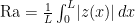
Thus, flat membranes have zero roughness, while patterned membranes with tall peaks and deep valleys have high roughness. A term called roughness normalized to pattern height (Ra_h) is defined as R_a/h, which helps quantify the percentage of the elevated area.

The chosen membrane performance indicator was boundary layer thickness (δ) calculated through Equation (10).

—- eq(10)

Overall, a linear correlation between roughness and boundary layer thickness was observed. Fig. 15a shows the data for all the geometries grouped by pattern size; boundary layer thickness correlated with roughness in each set. Fig. 15b shows the average of all the data in Fig. 15a and again a strong correlation exists. This finding supports the hypothesis that adding patterns onto membranes results in increased boundary layer thickness, decreased mass transfer, and therefore increased CP. This makes sense in light of the classical flat-plate boundary layer model [34]. Tangential flow results in solute being swept away from the surface, but with patterns present solutes in the valleys are shielded from the sweeping fluid. The net effect is that the greater the roughness the greater the boundary layer thickness.

Fig. 15. Roughness normalized to pattern height (Ra_h) versus boundary layer thickness (δ). (a) Five data series on the same plot corresponding to five sizes for each geometry. (b) Average value of the five data sets in (a).

In predicting performance for future patterned membranes, it may be possible to estimate CP based on the roughness without running full CFD simulations. Alternatively, pattern designs may exist that alter the hydrodynamics in creative ways resulting in a breakdown in the roughness vs. boundary-layer-thickness correlation; data would then fall under the line in Fig. 15b resulting in better water flux.

One possible way to break down the roughness vs. boundary-layer-thickness correlation is to change the flow orientation for the line-and-groove patterns. This is somewhat challenging using our current simulation techniques because repeating boundary conditions cannot be used for all flow orientations; however, we were able to add new simulations at the end of the study to evaluate the parallel flow case for rectangular line-and-groove patterns. We modified Fig. 15 to include the new results and we show those in Fig. S4. The parallel flow orientation did decrease the average boundary layer thickness by about 9%, but this is still not far from the correlation line. CP values in flat membranes were still lower than CP values in parallel flow line-and-groove patterns. Future work should explore novel geometries that might cause interesting flow disruptions to break the roughness vs. boundary-layer-thickness trend.

4. Conclusions

Patterned membranes with various shapes were studied for their potential to affect CP in RO membrane processes. A multi-scale modeling approach was used to enable investigation of a wide pattern size range. Velocity profile, concentration, shear stress, and permeate flux were evaluated. A Sherwood correlation fit the simulation results, affirming that the models were behaving rationally. None of the patterns decreased CP, although vortices were discovered near the membrane surface. Others have postulated that vortex formation would result in decreased mass buildup, but that was not the case for these laminar-flow simulations representing the regime that would exist for actual RO operations. Vortices that did form had low velocity so were not able to effectively scour the membrane surface. The mechanism for increased CP was related to roughness: increased roughness caused thicker boundary layers, and thus decreased the mass transfer coefficient.

An increase in CP caused a decrease in local water flux, as would be expected from the enhanced osmotic pressure in the CP layer. However, using a projected-area calculation (which is more relevant to full-scale systems) resulted in greater water flux in patterned membranes than flat membranes. The additional surface area provided by the patterns counteracted the exacerbated CP to yield an overall greater water throughput. This suggests that in experimental work that has shown patterned membranes performing better than flat membranes, the extra surface area resulting from patterning might be the reason that nominal flux was increased.

5. CRediT authorship contribution statement

Zuo Zhou: Conceptualization, Methodology, Software, Validation, Formal analysis, Writing – original draft, Writing – review & editing, Visualization.

Bowen Ling: Conceptualization, Writing – review & editing. Ilenia Battiato: Conceptualization, Writing – review & editing, Funding acquisition.

Scott M. Husson: Conceptualization, Writing – review & editing, Funding acquisition.

David A. Ladner: Conceptualization, Methodology, Formal analysis, Writing – review & editing, Visualization, Supervision, Funding acquisition.

6. Declaration of competing interest

The authors declare that they have no known competing financial interests or personal relationships that could have appeared to influence the work reported in this paper.

7. Acknowledgements

The authors gratefully acknowledge funding through the Designing Materials to Revolutionize and Engineer our Future (DMREF) program of the U.S. National Science Foundation, grant number 1534304. We also acknowledge computational support through the Palmetto Cluster, Clemson University’s primary high-performance computing resource.

8. References

[1] E.M. Vrijenhoek, S. Hong, M. Elimelech, Influence of membrane surface properties on initial rate of colloidal fouling of reverse osmosis and nanofiltration membranes, J. Membr. Sci. 188 (2001) 115–128, https://doi.org/10.1016/S0376-7388(01)00376-3.
[2] E.M.V. Hoek, A. Subir Bhattacharjee, M. Elimelech, Effect of Membrane Surface Roughness on Colloid− Membrane DLVO Interactions, 2003, https://doi.org/10.1021/LA027083C.
[3] Q. Li, Z. Xu, I. Pinnau, Fouling of reverse osmosis membranes by biopolymers in wastewater secondary effluent: Role of membrane surface properties and initial permeate flux, J. Membr. Sci. 290 (2007) 173–181, https://doi.org/10.1016/j.memsci.2006.12.027.
[4] M.R. Chowdhury, J. Steffes, B.D. Huey, J.R. McCutcheon, 3D printed polyamide membranes for desalination, Science (80-.) 361 (2018) 682–686, https://doi.org/10.1126/science.AAR2122.
[5] Y.J. Won, J. Lee, D.C. Choi, H.R. Chae, I. Kim, C.H. Lee, I.C. Kim, Preparation and application of patterned membranes for wastewater treatment, Environ. Sci. Technol. 46 (2012) 11021–11027, https://doi.org/10.1021/es3020309.
[6] S.Y. Jung, Y.-J. Won, J.H. Jang, J.H. Yoo, K.H. Ahn, C.-H. Lee, Particle deposition on the patterned membrane surface: simulation and experiments, Desalination 370 (2015) 17–24, https://doi.org/10.1016/j.desal.2015.05.014.
[7] Y.-J. Won, S.-Y. Jung, J.-H. Jang, J.-W. Lee, H.-R. Chae, D.-C. Choi, K. Hyun Ahn, C.-H. Lee, P.-K. Park, Correlation of membrane fouling with topography of patterned membranes for water treatment, J. Membr. Sci. 498 (2016) 14–19,https://doi.org/10.1016/j.memsci.2015.09.058.
[8] Y.K. Lee, Y.J. Won, J.H. Yoo, K.H. Ahn, C.H. Lee, Flow analysis and fouling on the patterned membrane surface, J. Membr. Sci. 427 (2013) 320–325, https://doi.org/ 10.1016/j.memsci.2012.10.010.
[9] S.T. Weinman, S.M. Husson, Influence of chemical coating combined with nanopatterning on alginate fouling during nanofiltration, J. Membr. Sci. 513(2016) 146–154, https://doi.org/10.1016/j.memsci.2016.04.025.
[10] O. Heinz, M. Aghajani, A.R. Greenberg, Y. Ding, Surface-patterning of polymeric membranes: fabrication and performance, Curr. Opin. Chem. Eng. 20 (2018) 1–12, https://doi.org/10.1016/J.COCHE.2018.01.008.
[11] B. Ling, I. Battiato, Rough or wiggly? Membrane topology and morphology for fouling control, J. Fluid Mech. 862 (2019) 753–780, https://doi.org/10.1017/jfm.2018.965.
[12] S.H. Maruf, A.R. Greenberg, J. Pellegrino, Y. Ding, Fabrication and characterization of a surface-patterned thin film composite membrane, J. Membr.Sci. 452 (2014) 11–19, https://doi.org/10.1016/j.memsci.2013.10.017.
[13] E. Lyster, Y. Cohen, Numerical study of concentration polarization in a rectangular reverse osmosis membrane channel: permeate flux variation and hydrodynamic end effects, J. Membr. Sci. 303 (2007) 140–153, https://doi.org/10.1016/j.memsci.2007.07.003.
[14] S.S. Sablani, M.F.A. Goosen, R. Al-Belushi, M. Wilf, M.F.A. Goosena, M. Wilf, Concentration polarization in ultrafiltration and reverse osmosis: a critical review, Desalination 141 (2001) 269–289.
[15] I. Sutzkover, D. Hasson, R. Semiat, Simple technique for measuring the concentration polarization level in a reverse osmosis system, Desalination 131(2000) 117–127, https://doi.org/10.1016/S0011-9164(00)90012-2.
[16] W.F. Blatt, A. Dravid, A.S. Michaels, L. Nelsen, Solute polarization and cake formation in membrane ultrafiltration: causes, consequences, and control techniques, in: Membr. Sci. Technol, Springer US, Boston, MA, 1970, pp. 47–97, https://doi.org/10.1007/978-1-4684-1851-4_4.
[17] M.C. Porter, Concentration polarization with membrane ultrafiltration, Ind. Eng. Chem. Prod. Res. Dev. 11 (1972) 234–248, https://doi.org/10.1021/i360043a002.
[18] E. Matthiasson, B. Sivik, Concentration polarization and fouling, Desalination 35 (1980) 59–103, https://doi.org/10.1016/S0011-9164(00)88604-X.
[19] T.H. Chong, F.S. Wong, A.G. Fane, Enhanced concentration polarization by unstirred fouling layers in reverse osmosis: detection by sodium chloride tracer response technique, J. Membr. Sci. 287 (2007) 198–210, https://doi.org/10.1016/j.memsci.2006.10.035.
[20] S. Kim, S. Lee, E. Lee, S. Sarper, C.-H. Kim, J. Cho, Enhanced or reduced concentration polarization by membrane fouling in seawater reverse osmosis (SWRO) processes, Desalination 247 (2009) 162–168, https://doi.org/10.1016/j.desal.2008.12.021.
[21] A.L. Zydney, Stagnant film model for concentration polarization in membrane systems, J. Membr. Sci. 130 (1997) 275–281, https://doi.org/10.1016/S0376-7388(97)00006-9.
[22] S. Kim, E.M. V Hoek, Modeling concentration polarization in reverse osmosis processes, Desalination 186 (2005) 111–128, https://doi.org/10.1016/j.desal.2005.05.017.
[23] R. Ranjan, S. DasGupta, S. De, Mass transfer coefficient with suction for laminar non-Newtonian flow in application to membrane separations, J. Food Eng. 64 (2004) 53–61, https://doi.org/10.1016/j.jfoodeng.2003.09.012.
[24] T. Ishigami, H. Matsuyama, Numerical modeling of concentration polarization in spacer-filled channel with permeation across reverse osmosis membrane, Ind. Eng. Chem. Res. (2015), https://doi.org/10.1021/ie5039665.
[25] P. Xie, L.C. Murdoch, D.A. Ladner, Hydrodynamics of sinusoidal spacers for improved reverse osmosis performance, J. Membr. Sci. 453 (2014) 92–99, https://doi.org/10.1016/j.memsci.2013.10.068.
[26] C.Y. Tang, Y.-N. Kwon, J.O. Leckie, Fouling of reverse osmosis and nanofiltration membranes by humic acid—effects of solution composition and hydrodynamic conditions, J. Membr. Sci. 290 (2007) 86–94, https://doi.org/10.1016/j.memsci.2006.12.017.
[27] J.H. Jang, J. Lee, S.-Y. Jung, D.-C. Choi, Y.-J. Won, K.H. Ahn, P.-K. Park, C.-H. Lee, Correlation between particle deposition and the size ratio of particles to patterns in nano- and micro-patterned membrane filtration systems, Separ. Purif. Technol. 156 (2015) 608–616, https://doi.org/10.1016/j.seppur.2015.10.056.
[28] M. Mulder, Basic Principles of Membrane Technology, Kluwer Academic Publishers, Boston, 1991.
[29] V. Gekas, B. Hallstrom, Mass transfer in the membrane concentration polarization layer under turbulent cross flow. I. Critical literature review and adaptation of existing Sherwood correlations to membrane operations, J. Membr. Sci. 30 (1987) 153–170, https://doi.org/10.1016/S0376-7388(00)83069-0.
[30] P. Xie, L.C. Murdoch, D.A. Ladner, Mitigating Membrane Fouling with Sinusoidal Spacers, Desalin. Water Treat., Submitted, 2019.
[31] M.M. Clark, Transport Modeling for Environmental Engineers and Scientists, second ed., WILEY, 2009.
[32] U. Ghia, K.N. Ghia, C.T. Shin, High-Re solutions for incompressible flow using the Navier-Stokes equations and a multigrid method, J. Comput. Phys. 48 (1982) 387–411, https://doi.org/10.1016/0021-9991(82)90058-4.
[33] T.R. Thomas, Characterization of surface roughness, Precis. Eng. 3 (1981) 97–104, https://doi.org/10.1016/0141-6359(81)90043-X.
[34] R.B. Bird, W.E. Stewart, E.N. Lightfoot, Transport Phenomena, J. Wiley, 2007.