Modeling Powerbus and Cable with HFSS (version 11.1.3)
|
Geometry and setup |
Double-sided PCB:
- Size: 125 mm × 100 mm × 1 mm
- Top and bottom metal: PEC
- Dielectric: FR4, εr = 4.5,
dielectric loss tangent = 0.015
Cable (round cable):
- Length: 1000 mm
- Radius: 2 mm
- Material: PEC
Excitation:
Voltage source (1 V, 50 ohms)
Boundary:
Radiation, Infinite ground
Analysis
Setup:
- Solution Frequency: 300 MHz (<300 MHz), 1.8 GHz (>300 MHz)
- Maximum Number of Passes: 50
- Maximum ΔS: 0.01
- Do Lambda Refinement: 0.3
- Maximum Refinement Passes: 20%
Sweep:
- Sweep type: Discrete
- Frequency Setup: 10 MHz - 2 GHz, Step Size =
10 MHz
 hfss_powerbus_cable.zip
|
|
Simulation result |
Simulation Time: 11 mins(<
300 MHz) + 39 mins (> 300 MHz)
Number of passes
completed: 7
Number of tetrahedra: 10961
|
|
Decisions the user must make that affect the
accuracy of the result |
- Infinite ground plane: assign the bottom face of the radiation
boundary to infinite ground plane with perfect E boundary
- Location of absorbing boundary: for low frequencies (<300
MHz), use a large radiation boundary (radius = 1562.5 mm). For high
frequencies (>300 MHz), use a small radiation boundary (radius
= 212.5 mm).
- Maximum ΔS: default = 0.02, this model = 0.01
- Do lambda refinement: default = 0.333, this model =0.3
- Cable model: use flat ribbon instead of round cable
|
|
Comments |
- How did the location of the
absorbing boundary affect the result at low frequencies?
Two meshes were used to model this problem. At high frequencies
(> 300 MHz), the ground plane had a diameter of 212.5 mm, and
was terminated at the absorbing boundary. At low frequencies (< 300
MHz), the ground plane had a diameter of 1562.5 mm in order to put
the absorbing boundary sufficiently far from the object being
modeled.
More information
...
- How did we define the wire?
We used a flat ribbon to model the 1-m cable. HFSS also allows
us to model the cable as a round wire.
More information
... | |
Screen shots
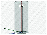
Fig. 1. Simulation model
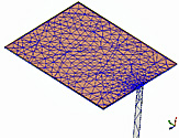
Fig. 2. Simulation meshes
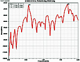
Fig. 3. Electric field at 10 m,
θ=0°, φ=0°
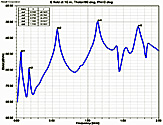
Fig. 4. Electric field at 10 m,
θ=90°, φ=0°
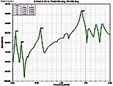
Fig. 5. Electric field at 10 m,
θ=90°, φ=90°
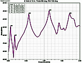
Fig. 6. Electric field at 10 m,
θ=90°,
φ=180° | |
)
)
)
)
)
)