Weiming Qi and David A. Ladner
Published in the Journal of Environmental Engineering.
Cite as: Qi, W.; Ladner, D.A. “Automated testing apparatus for ceramic membrane filtration of high-strength industrial wastewater.” Journal of Environmental Engineering 2023, 149, 04023063. https://doi.org/10.1061/JOEEDU.EEENG-7337

Abstract
A common problem in scale-up of membrane filtration research from the laboratory to industrial practice is that the testing methods used in the laboratory are often quite different than full-scale industrial applications. Lab-scale experiments usually test membranes in single filtration steps using manual systems, while industrial applications use membranes with frequent backwash and clean-in-place (CIP) steps. This is especially true for high-strength industrial wastewater applications where frequent backwash and CIP steps are needed to maintain membrane flux; the behavior of the membrane in such applications can be different than the behavior of the virgin material used in the lab. An automated membrane filtration apparatus built in our lab helps to solve this problem by allowing long-term filtration, frequent backwash and CIP, and high-accuracy operation. The filtration system achieves different cleaning strategies for both theoretical research and practical water and wastewater scale-up experiments. The embedded control algorithms achieve operational accuracy in terms of maintaining flux and/or trans-membrane pressure (TMP) at their desired set points. A flux-step function enables operators to measure critical flux automatically. The filtration system handles a variety of microfiltration and ultrafiltration membranes in crossflow or dead-end mode with backwash integration, CIP capability, and aeration scouring. Synthetic rendering wastewater and raw rendering wastewater were applied to test the apparatus in the lab and in the field, respectively. The control algorithms successfully dampened oscillations using custom calibration curves. Three backwash-CIP strategies were tested with both wastewater types. The first was time triggered backwash and cycle number triggered CIP, which resulted in stable and reliable operation, but required close operator control and thus was not fully automated. The second strategy was time triggered backwash with TMP triggered CIP, which responded quickly to water quality fluctuations and achieved full automation, but the TMP target had to be carefully decided to enhance the efficiency of CIP. The third strategy was target-TMP backwash with duration triggered CIP, which can achieve the most advanced and flexible filtration system, though setting up this level of automation complexity in the field was challenging. Both backwash and CIP frequencies responded to real-time performance automatically. Ultimately, the automated lab-scale filtration apparatus operated similarly to full-scale systems, which should help fill the gap between laboratory research and scale-up of industrial applications.
1. Background
Membrane technology is widely used in industrial applications of water and wastewater treatment; however, membrane fouling increases the resistance to water flow and decreases productivity, which increases the operational cost and limits the filtration performance (Ezugbe and Rathilal 2020; Hube et al. 2019). Membrane fouling is a particularly egregious challenge in high-strength industrial wastewater such as in the rendering industry where waste streams have high concentrations of fats, oils, and grease (FOG) (Zhou et al. 2015). With high-strength wastewater, frequent backwash and clean-in-place (CIP) steps are needed to maintain membrane flux. Most studies of membrane fouling in the literature focus on the filtration step; it is much less common to find experiments where the backwash and CIP steps are included. This is a problem for high-strength wastewater applications because the behavior of the membrane material in the context of backwash and CIP may be much more important than the behavior of the material in one short filtration-only test. For example, ultrafiltration shows much better fouling reversibility during filtration of proteins compared with microfiltration, which requires experiments having multiple filtrations with backwash and CIPs (Marshall et al. 1993). Unfortunately, testing membranes in the laboratory with multiple cycles of filtration, backwash, and CIP is laborious. An automated system would be useful to accomplish such work.
The high concentrations of FOG in rendering wastewater make classical primary clarifier treatment less effective. Dissolved air floatation (DAF) has a higher efficiency than primary clarification for removing fats and proteins, thus making DAF the most often used primary treatment method; DAF is employed in approximately 80% of slaughterhouse wastewater plants in the U.S. (Abboah-Afari and Kiepper 2012; Al-Mutairi et al. 2008; Johns 1995). One main problem with DAF is that the fats and proteins (which are recoverable and valuable products) are degraded during aggressive aeration with micro-size bubbles (Lo et al. 2005). The caustic and acid used for adjusting pH before DAF also increase the operational cost. To enhance the efficiency of aggregation and material removal, coagulants and flocculants are necessary (Bustillo-Lecompte and Mehrvar 2015). These additives are undesirable because they reduce the value of the recovered fat and protein stream. Operational challenges occur in DAF when the wastewater quality fluctuates. Close control, skilled operators, and customized chemical additives are often required to make DAF feasible (Cheryan and Rajagopalan 1998).
Membrane technology can be an efficient alternative to DAF with better effluent quality (Avula et al. 2009; Racar et al. 2017; Wandera and Husson 2013; Yordanov 2010; Zhou et al. 2015). Membranes can be operated without coagulants and flocculants so these chemicals will not be retained and will not affect the product stream, though caustic and acid are required to clean the membrane periodically for maintaining flux. The main limitation with membranes is fouling, which reduces filtration performance and increases operational cost (Mohammad et al. 2012). Fouling is more severe for FOG wastewater than for other industrial and municipal wastewaters. The properties of the membrane surface can mitigate membrane fouling from some of the constituents, such as hydrophilic surfaces decreasing fouling tendency from oil droplets (Tummons et al. 2020), but proteins in FOG wastewater are zwitterions which causes high fouling tendency even for membranes with hydrophilic surfaces (Maximous et al. 2009). High frequency of backwash and CIP is more important for treating FOG wastewater compared with other wastewater types; this amplifies the importance of system automation for FOG applications.
Lab-scale filtration experiments of FOG wastewater from the literature usually employ manual systems without automation. It is rare to find published performance studies that include backwash steps and even rarer to find those that incorporate CIP steps. (When membranes are cleaned between experiments, they are usually removed from the system and cleaned manually.) Treatment of poultry processing wastewater (PPW) with ultrafiltration membranes was studied to optimize the filtration performance with pH of 5.5 – 7, flow rate of 600-800 ml min-1, and TMP of 10 – 14 psi, without any backwashes and CIPs (Lo et al. 2005). Polyacrylonitrile, polysulfone, and polyvinylidene difluoride membranes have been tested for PPW with pressures of 50 to 80 psi to minimize the membrane fouling without any online cleaning process (Abboah-Afari and Kiepper 2012). The reuse of rendering plant wastewater was carried out with three ultrafiltration membranes, two nanofiltration membranes, and one reverse osmosis membrane. Permeate water quality and fouling tendency were the parameters evaluated without any cleaning procedures (Racar et al. 2017). PPW was filtered with an ultrafiltration membrane at a pressure of 40 psi and crossflow rate around 1 m/s to recover a nutritional by-product. Backwashes and CIPs were not mentioned during the economic evaluation of net revenue from by-product recovery. Some other papers mention their cleaning process for removing the fouling between experiments but do not focus on cleaning procedures in their laboratory analysis (Wandera and Husson 2013; Zhou et al. 2015). To understand whether the results of these published studies of FOG wastewater will be meaningful at full scale, backwash and CIP steps would need to be incorporated into pilot experiments.
The gap between lab experiments and industrial applications occurs because industrial wastewater requires frequent backwash and CIP. An automated filtration system is usually employed for industrial application. In contrast, backwash and CIP are challenging to accomplish in lab studies because most experiments are performed manually or with partial automation. An operator must be present to induce filtration and backwash, and chemical cleaning is often done by removing the membrane from the system and cleaning by hand. These procedures increase the labor load and cause investigators to keep their experiments short; many fouling tests reported in the literature are completed in a few hours. To mimic real systems that operate for days and weeks, (or even just for an over-night experiment) automation is needed.
Manual operation also influences the operational accuracy. For example, flux from low-pressure membrane is sensitive to transmembrane pressure (TMP). When a peristaltic pump is applied to pull out the permeate, a real-time correction is necessary to maintain the permeate flowrate as the TMP increases. For most experiments with peristaltic pumps for permeate suction, there was no calibration of the pump speed as the TMP increased (Cho and Fane 2002; Clech et al. 2003; Defrance and Jaffrin 1999; Kim and DiGiano 2006). On the other hand, when TMP is required to be maintained, the peristaltic pump should be corrected to pull out less permeate for maintaining the TMP because of the accumulation of membrane fouling. This is impossible for an operator to precisely control because of the fine and frequent adjustments needed.
This paper aims to fill the gap between laboratory testing methods and full-scale operational methods by introducing an automated filtration system in detail. Here is described the basic control logic, the hardware setup, programming the control system in LabVIEW, and challenges overcome when combining components to achieve a complete unit. The filtration system allows a variety of operational modes for membrane scale-up research. Filtration, backwash, and CIP can be triggered by different strategies. Crossflow, aeration, and the flux-step functions are also included for membrane challenge experiments. Unique algorithms in the data acquisition and control software successfully dampen oscillations that would otherwise occur when automatically controlling pump speed to target a particular flux or TMP. All functions were tested in our lab using synthetic wastewater and in the field using high-strength industrial wastewater at a rendering plant.
2. Methods – system setup
The membrane filtration system designed here aims to fulfill the requirements of membrane filtration experiments that seek to mimic industrial practice. During the operation process, filtration, backwash, and CIP are essential steps. All steps are executed with hardware like pumps and solenoid valves. The trigger of each action is controlled and monitored with a software program. Fig. 1a shows a photo of the filtration system.

2.1 Hardware
The system hardware can be divided into three types: basic components, fluid-handling hardware, and electronic interface. Fig. 2 shows the schematic of the membrane system.

2.1.1. Basic components
The frame of the membrane unit was built with T-slotted structural framing material (also called “80/20” extruded aluminum) and associated parts like brackets, hinges, connectors, plexiglass, and casters. We use the term “pallet-size” for the system because it is small enough to transport with a pickup truck and is easily moved with a forklift. For added mobility we made the width small enough to fit through typical doorways and we added castors so it can be rolled. The pallet unit has two tiers. The lower tier is for liquid-processing components, and the upper tier houses electrical components. A desktop computer (#1 in Fig. S1) mounted on the upper tier is for controlling all electrical components. An uninterrupted power supply (UPS) (#2 in Fig. S1) was employed on the upper tier to make sure the system ran stably because we found the computer might shut down at the moment that several solenoid valves were adjusted together, which drew a high current. A light and a video webcam were mounted to illuminate and visualize the lower tier, which enabled the operator to monitor the fluid-handling hardware day and night.
2.1.2 Electrical interface and sensors
Most electrical components were centralized in a panel (Fig. 1b) at the front of the unit on the upper tier since we could easily access it and protect it from water spills. Three A/C to DC power transformers (#1 in Fig. 1b) at the top of the front panel provided power to the transmitters and transducers. Other visible components were wired to conduits and terminal blocks.
Different transducers and transmitters were employed to translate sensor signals to electrical outputs. Two multifunction I/O devices (National Instruments Serial Interface Device USB – 232/4, #3 in Fig. 1b) received RS-232 signals from serial ports and delivered them to the computer through a USB interface. These controlled three pumps and received electrical readings from the flowmeter and the balance. NI cDAQ-9171 and NI 9482 (#4 in Fig. 1b) worked together to receive signals from the computer and switch solenoids on and off. A pH transmitter (αpH 500, #5 in Fig. 1b) transferred the pH values to electrical output (4-20 mA), and a conductivity transmitter (#6 in Fig. 1b) and temperature transmitter converted conductivity and temperature values to electrical outputs.
2.1.3 Fluid-handling hardware
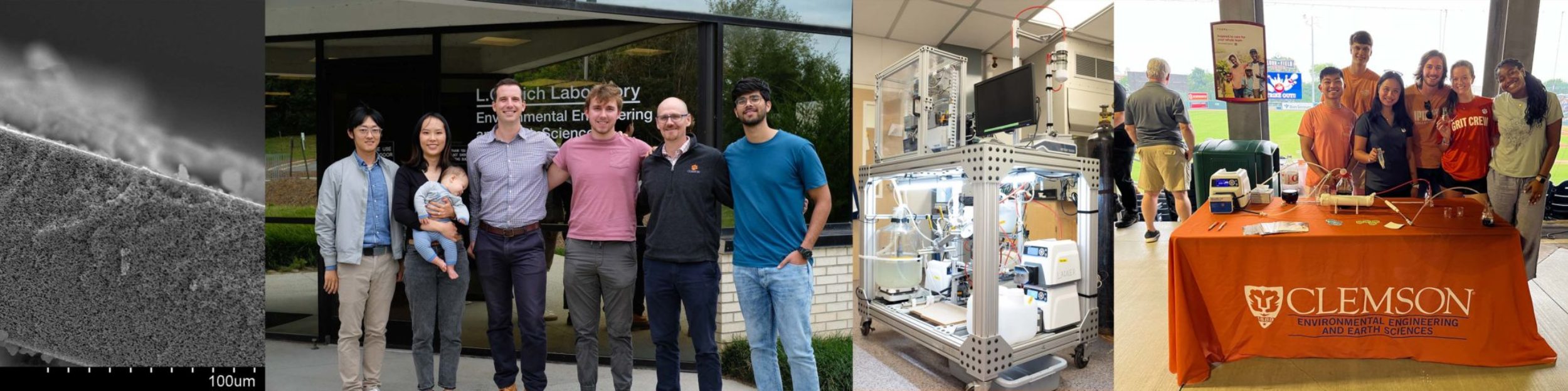
The fluid-handling hardware carried out the different filtration steps. Tubular ceramic membranes (Al2O3) fabricated by Inopor had mean a pore size of 100 nm and effective membrane area of 0.025 m2 (Fig. 3b). The membrane housing (Fig. 3a) was a 316-stainless steel cell with feed, concentrate, backwash, and permeate ports. Four manual ball valves were installed on four ports to easily unload the membrane module after the experiment.

The flat-sheet membrane (Fig. 3d) fabricated by Meidensha had mean pore sizes of 100 nm. A membrane housing was built with acrylic plastic to hold the membrane to create crossflow and scouring. There were four ports on the membrane housing, which were for feed, concentrate, permeate outlet/cleaning inlet, and gas inlet. An air stone on the bottom of the housing connected with a gas inlet provided air scouring.
Three peristaltic pumps (Fig. 1c P1, P2, and P3) were installed for creating feed flow, permeate suction, and chemical cleaning/backwash flow, respectively. Four solenoid valves (Fig. 1c -S1, S4 and Fig. 1d-S2, S3) were employed to control the flow entering or leaving the module during filtration, backwash, and chemical cleaning. The first solenoid valve was on the permeate port. During backwash or chemical cleaning, this port would close for blocking the flow to induce high pressure. The second and third solenoid valves were for controlling backwash and chemical cleaning, respectively. The fourth solenoid valve was a three-way valve, which was used for waste control. During chemical cleaning, chemical contamination was produced, which degraded the FOG wastewater. In this case, the chemical waste would not go back to the feed tank but to the waste tank, which was controlled by the fourth solenoid valve.
Two pressure sensors (b – PS1, PS2) were installed to measure the pressure at the concentrate port and backwash/cleaning port. A differential pressure sensor (Fig. 1d – D) was used to monitor the differential pressure between the feed and permeate sides. A balance was mounted in the flow path before the permeate tank. A self-emptying device (Fig. 4) was placed on the balance. The device accumulated permeate to 300 ml and then the permeate was emptied automatically via a siphon mechanism. Permeate inlet flow and outlet flow were driven by gravity and the self-emptying device did not touch any other components, which made the balance readings more precise. Mass measurements over time were used to calculate permeate flow rate and membrane volumetric flux.

Four carboys worked as feed tank (Fig. 1c-T1), permeate tank (Fig. 1c-T3), chemical tank (Fig. 1c-T2), and waste tank, respectively. A spill port was installed in the permeate tank; when the water level reached the spill port the permeate flowed into a collection tank, back to the feed tank, or to a waste tank, depending on the experiment being performed.

2.2. Software
A control system was coded in LabVIEW for data acquisition and system control. The fundamental structure of the program was a while loop that iterated continuously until a stop signal was sent by the user or a task was finished. One iteration usually lasted less than one second, depending on how many functions were running during each iteration. For example, a loop that sent an email or wrote data to disk took more time than a normal loop.
2.2.1. Operational steps algorithm
Eight steps were created to fulfill the filtration requirements. Four of them were the main steps for filtration, backwash, CIP, and residual removal. Before each main step, there were four preparation steps, respectively, to set up the system for each subsequent main step. Each step was programmed into one case structure in LabVIEW, numbered from one to eight, respectively. The case selector was connected to the step selection algorithm, which used real-time data (TMP and time) to decide which step to activate.
2.2.1.1. Preparation steps
The preparation steps reset the system from the previous steps and made the system ready for the following main steps. Sequence structures were created in LabVIEW for each preparation step (step one, three, five, and seven) because a sequence structure contained one or more frames that were executed in sequential order. Usually, all the preparation steps had the frames in the sequence structures to reset all three pumps and five solenoid valves. Then, setup frames were executed to make the system ready for the following steps. These frames turned on specific pumps; for example, the filtration step needed the feed and suction pumps activated, but the backwash step needed the feed and backwash pumps activated. Solenoid valves were also switched according to the desired water flow path for the following main step.
Preparation steps also had other functions to ensure that the following main step operated correctly. In step one, there was one special frame to fill the permeate chamber with a negative backwash pump speed (-10% of normal backwash pump speed) for three seconds to decrease the time that step two (filtration) required to reach a stable TMP. In step five and seven (the preparation steps for CIP and residual removal), two frames were used to fill or remove chemical inside the membrane and the tubing. Usually, preparation steps took 60 seconds each, which meant some frames in the sequence structures were empty frames with wait functions. A wait function was also applied to all reset and setup frames to ensure enough time for the system to execute all of the actions. Steps five and seven needed more time than other preparation steps because the backwash pump took 65 seconds to fill the membrane and tubing with a certain volume, around 150 ml.
2.2.1.2. Main steps
The main steps (steps two, four, six, and eight) followed preparation steps (steps one, three, five, and seven). The bulk of time spent on filtration, backwash, CIP, and residual removal occurred during the main steps. The duration of one main step was flexible and users could set it up before the filtration process. The purpose of the main steps was to adjust the system in response to the filtration performance data. Preparation steps set up and initiated all the operations and parameters except the pump speed, which was adjusted during the main steps to control the filtration, backwash, CIP, and residual removal.
Step two was the filtration step, in which the filtration flux (or TMP) was adjusted to meet its set point. For example, the filtration flux was physically controlled by suction pump speed and the TMP increased along with constant flux filtration due to fouling accumulation. When constant TMP was required, the suction pump speed was adjusted automatically to maintain the TMP.
The critical flux or TMP is important for membrane filtration operation. The system had a built-in flux-step /TMP-step function to measure the critical flux/TMP. In this case, the target filtration flux or TMP was not constant; a program in step two could adjust the flux or TMP automatically. Backwash or even CIP could be applied between filtrations, which made the critical flux measurement more precise.
Pressure maintenance happened in steps four and eight (backwash and residual removal steps). Backwash with high flux is more effective at removing accumulated material (Vera et al. 2015), but the aggressive backwash may damage the membrane. For this reason, the TMP was monitored, and the backwash pump speed was adjusted accordingly so that the TMP reached its user-defined set point.
2.2.2. Step selection algorithm
A step selection algorithm was coded to control the case structure with eight steps. The step selection algorithm decided when one step should be ended by different criteria. All preparation steps had pre-set durations, which meant the step selection algorithm would finish them with accumulated time as criteria. Ending the filtration step (the second step) was the most important part of this program since the filtration step was usually followed by steps three and four (backwash preparation step and backwash step). On the other hand, the trigger of CIP was also related to the performance in the filtration step. This program was designed with two methods to trigger the backwash and three methods to start the CIP (described below).
Three cleaning strategies were designed based on different combinations of backwash and CIP triggers. Table 2 shows the strategies and triggers employed. Each trigger is described below. Some trigger combinations were meaningless, such as TMP triggered backwash and TMP triggered CIP; those are not included in the table.

All strategies were packed into one sub-program. The basic logic was a case structure which used pre-set values and filtration data to decide the output numbers for the steps. Relative time was the most important reference to end all preparation steps and time-based main steps. The accumulation time of these steps was calculated using relative time at the beginning of each step. When the accumulated time reached the pre-set level, the next step would be triggered.
2.2.2.1. Time triggered backwash
Time is the most common trigger during membrane filtration in the research and industrial world because data analysis is not required. The benefit of a time-based trigger was that the control algorithm was simple and usually error free. However, the system could not respond dynamically to factors like feed-water quality, membrane fouling behavior, or ambient temperature. Backwash was triggered by filtration duration in Strategies 1 and 2, as shown in Fig. 5a and Fig. 5b, respectively. Lines are added to the figures to represent reversible fouling, irreversible fouling, and residual fouling (Wang et al. 2014).

2.2.2.2. TMP triggered backwash
In constant flux operation TMP represents the fouling behavior of the membrane, which makes the TMP trigger an appropriate adaptive control. The TMP trigger limited the fouling behavior and avoided damaging the membrane. Signal noise challenged the TMP trigger since some extreme value led to unexpected backwashes. A moving average filter was applied to reduce noise. As shown in Fig. 5c, the TMP never goes above the trigger set point, thus protecting the membrane from pressure overload. The TMP trigger can increase the efficiency of filtration when the water quality is good and fewer backwashes are needed. However, a disadvantage is that testing is needed to carefully choose the TMP set point. If the set point is too low, backwash will occur frequently and filtration efficiency is reduced. If the set point is too high, the energy for filtration is increased and fouling may be exacerbated.
2.2.2.3. Cycle number triggered CIP
The cycle number trigger counts the number of backwash cycles and is usually applied with the time trigger backwash (Fig. 5a). This trigger is simple and relatively error free, but is not adaptive to filtration performance.
2.2.2.4. TMP triggered CIP
During the time triggered backwash, TMP triggered CIP can be applied (Fig. 5b). Backwash cannot remove all parts of the fouling so the TMP at the end of each filtration typically increases. When the TMP at the end of the filtration reaches a set point, CIP is triggered to recover the irreversible fouling. The benefit of this strategy is that the maximum TMP is predictable. The TMP limit protects the membrane from overload.
2.2.2.5. Duration triggered CIP
CIP can be triggered with filtration duration when backwash is triggered with TMP (Fig. 5c). In constant flux conditions, the irreversible fouling contributes to a higher TMP at the beginning of filtration, which leads to a shorter time to reach the TMP backwash trigger. Thus, the filtration time indicates the irreversible fouling on the membrane. When the irreversible fouling increases, the efficiency of filtration will decrease and CIP is necessarily carried out to remove the irreversible fouling and recover the TMP. The black line in Fig. 5 shows the irreversible fouling along with filtration time. When the irreversible fouling increases and filtration duration decreases, the CIP will be triggered to remove much of the irreversible fouling.
2.2.3. TMP and Flux Control Algorithm
The TMP and flux control algorithm works for creating constant TMP or flux by adjusting the suction pump speed. The suction pump used for pulling out the permeate can maintain the flowrate at low TMP; however, foulants in the wastewater increase the resistance of the membrane and lead to a growing TMP. The program adjusts the suction pump speed to maintain a constant TMP when the constant TMP mode is applied.
The same mechanism is used for maintaining the flux. In theory, the permeate flux is only related to the suction pump speed, no matter whether the fouling is accumulating; however, the tubing of the peristaltic pump can only maintain the flowrate at low-pressure conditions. That means a correction is necessary for the constant flux mode during high TMP filtration. The TMP and flux control algorithm adjusts the pump speed for a constant flux at different pressures.
The calibration curve [Figs. 6(a and b)] shows the difference between the measured and target TMP (△TMP) to the required change in suction pump speed. The adjusted pump speed is added to the old speed. There are four linear relationships in the curve. When the differential TMP is between
and 3 psi, there are higher slope values than other ranges to make sure the program is sensitive enough to respond to the fluctuations.
The two slopes in the second quadrant are lower than the fourth quadrant’s, which makes the TMP increase and decrease at different rates. This setup is important to stabilize the suction pump speed. A situation was experienced that the suction pump was always adjusted, and the target TMP was never reached. The problem was found as the rates of increasing and decreasing △TMPs had the same absolute value, which made the TMP always higher or lower than the acceptable range [Fig. 6(c)]. To avoid this situation, different slopes were applied as shown in Fig. 6(d) to ensure that the TMP would reach the acceptable range.
The TMP and flux control algorithm was also used for keeping backwash and chemical cleaning pressure stable. The program was similar but with different parameters because the pump-speed range was 0–100 rpm, and the backwash pressure was maintained at 35 psi.

2.2.4. Flux-Step Algorithm
Critical flux is the idea that below a certain flux, the TMP remains constant, whereas if this flux is exceeded, the TMP increases over time. Various flux-step procedures have been used by others to measure the critical flux for different types of membranes (Cho and Fane 2002; Clech et al. 2003; Çulfaz et al. 2011; Huang et al. 2008; Kwon and Vigneswaran 1998; Monclús et al. 2011; Mutamim et al. 2012, 2013; Vera et al. 2014; Wu et al. 2008). One conceptualization of critical flux identified two forms: strong and weak (Field and Pearce 2011). The strong form of critical flux does not have any additional sources of hydraulic resistance other than the membrane itself. The weak form of critical flux considers additional hydraulic resistance from fouling.
A flux-step procedure for evaluating critical flux involves successive filtration steps at different flux values while measuring TMP. The measured TMP is used to determine the fouling rate and the membrane resistance. An important issue with flux-step procedures is that fouling resistances from the previous steps often affect the following step and contribute to a lower calculated critical flux.
The flux-step function in the system is automated and inserts backwash between two filtrations to remove the reversible fouling. CIP can also be applied to the membranes between the filtrations to remove the irreversible fouling. With these cleanings, reversible and irreversible fouling are disregarded and a more accurate critical flux measurement can be obtained. Different filtration parameters like the duration of filtration, backwash and CIP, crossflow velocity, and strength of cleaning are flexible in determining the critical flux under various conditions.
2.2.5. Data Acquisition and Processing Algorithm
The testing apparatus records 22 groups of data in a CSV file every 10 s. The signals received from the sensors are voltage signals. Calibrations of pressure, pH, conductivity, and temperature transmitters are made to translate voltage signals to physical parameters. Calibration curves and calibration processes are shown in Fig. S2.
2.2.5.1. Data Averaging
A moving average filter is employed to enhance the stability of the system. For example, the TMP fluctuates during the filtration due to particles blocking the tubing and unstable flow from peristaltic pumps. When pressure control is used to maintain the TMP, this turbulence will bring extra adjustment to suction pump speed. This situation not only influences the experimental results by providing fluctuating values but also causes too-frequent adjustment and thus additional wear of the suction pump. To avoid this situation, the average of an array including several TMP values was calculated to represent the real-time TMP value. For each iteration, the averaging window shifts forward, which uses the latest TMP value to replace the oldest value in the window. The average values have much less variability and are thus better suited for the TMP and flux control program input. Data averaging is also employed during backwash to maintain backwash pressure for protecting the membrane from breaking.
2.2.5.2. Data Storage
In every iteration of the while loop, the program will check if the data should be saved, which is decided by the preset frequency. In the file-saving iteration, a new group of data will be written to the CSV file. However, when a high frequency is set (e.g., every 5 s), a large file will be created at the end of a long-term filtration (e.g., more than 10 days). The large-size file delays the system by increasing the duration of the file-saving iteration and introducing more errors to the filtration system. A separating and combining program was created, which generates a new file every 24 h and combines all files together at the end of one experiment.
2.2.5.3. Email Notifications and Alarms
Data files and a figure containing TMP and flux were sent to the operator every 3 h for monitoring. An alarm system was built to monitor the TMP and water level. When the TMP was higher or lower than the preset value, which meant there was blocking inside the tubing or valves, the system sent an email alert. The conductivity probe mounted at about half the height of the feed tank was used to monitor the water level. When there was a leak in the system, the water level decreased lower than the conductivity probe, and an alarm email would be sent.
2.2.6. Other Functions
2.2.6.1. Flowrate Calculation
Flowrate is calculated based on the self-emptying device on the balance. In a perfect world, the permeate water would continuously flow into the device and the change in weight over time would yield stable flowrate calculation. However, the permeate flow is not continuous but falls in drops due to surface tension and unsteady peristaltic pump pulsation. To smooth the variability, curve fitting was employed to find the slope between the weight reading and the relative time. Eight groups of weight-time data points from the last eight iterations were used to find the slope of a line through the data, which was the flow rate in ml/min. The more data points used, the stabler the flow rate calculation; on the other hand, a delay in response time also occurs. In the system, eight data points were typically used, which struck a balance between stability and response time.
2.2.6.2. Controlled Termination of Experiments
An auto-stop program and a resetting program were coded. The auto-stop program included three methods to finalize each experiment. The first was a manual Stop button on the front panel, the second was a setting to end after a desired time, and the third was a trigger to end the flux-step function after cycling through the desired TMP or flux values. As mentioned before, the whole program is in a while loop except a resetting program. When the while loop is stopped, the resetting program will reset all the hardware. The program sets all solenoid valves to default status, sets the actuator valve to fully open, stops the pumps, and sends an email with the data and flux figures.
2.3. Experiments to Evaluate Apparatus Performance
The membrane testing apparatus can handle all types of low-pressure–driven filtration. The system was tested with different kinds of water and wastewater (lake water, tap water, activated sludge, and rendering wastewater). Rendering wastewater challenged the system much more than other types of feed water and highlighted the need for automated backwash and CIP. The system was first tested in the lab with synthetic high-strength wastewater to evaluate its stability and reliability. The synthetic wastewater recipe was modified from one found in the literature (Ersahin et al. 2014). That recipe called for “macronutrients” and “micronutrients;” the recipe used only the macronutrients because these were expected to be the main foulants (Table S1). Six experiments were done with different experimental setups for the evaluation of system functions. All experiments used filtration permeate for backwash and pH 13 NaOH as the chemical agent for CIP. The backwash strength was controlled at 35 psi with the TMP control algorithm, and the CIP strength was nominally 9.7 LMH based on the pump speed (without flux control via an algorithm). The membrane was cleaned out of place between experiments. Then, the system was deployed to the rendering wastewater plant for further evaluation. All experimental parameters are listed in Table S2.
2.3.1. Experiment 1—Data Acquisition and Presentation
The data acquisition and processing algorithm was first tested after building the system because it was used to record all the data for the following experiments. The experiment was carried out with the synthetic wastewater with constant flux of 9 LMH. Cleaning Strategy 3 was applied with TMP-triggered backwash of 5 psi and duration-triggered CIP of 25 min. The duration of backwash was 30 s, and the duration of CIP was 30 min.
2.3.2. Experiment 2—Data Averaging
Data averaging was tested with various parameters to dampen the noise from the differential pressure transmitter and the flowmeter. Experiment Two tested the implementation of a moving average with a window size of 1, 5, 10, 15, 20, 25, and 30 data points, respectively, to figure out the best averaging parameter. The experiment used synthetic wastewater for constant TMP filtration (
2.3.3. Experiment 3—Flux Control Algorithm
The parameters contributing to the flux control algorithms were tested with the synthetic wastewater as an example to avoid undamped oscillations. A special calibration curve was juxtaposed with an example of an uncalibrated curve based on the treatment of synthetic wastewater with constant flux filtration (
2.3.4. Experiment 4—Flux-Step Algorithm
Experiment 4 was carried out to test the critical flux of the synthetic wastewater with target flux from 6–30 LMH with a step height of 2 LMH. Strategy 1 was applied with time-triggered backwash every 30 min without CIP. Backwash was applied at the end of each step for 30 s with a strength of 35 psi to remove reversible fouling, which was recommended as a better alternative to the common flux-step method that does not use backwash between steps (Van der Marel et al. 2009). The crossflow velocity was relatively low at 0.0045 m/s compared to other published work (Barati et al. 2021; Chang et al. 2014; Zhou et al. 2015), which probably contributed to a lower critical flux.
2.3.5. Experiment 5—Cleaning Strategy
In Experiment 5, three cleaning strategies were tested with the synthetic wastewater. Refer to Table 2 for general information about each strategy. Strategies 1, 2, and 3 were tested with synthetic wastewater with constant flux filtration. The flux was 12 LMH for Strategies 1 and 2 and 10 LMH for Strategy 3 because of the accumulation of membrane fouling. Backwash was triggered every 15 min in Strategies 1 and 2 with a duration of 30 s. Strategy 3 triggered backwash with a TMP target of 6 psi. Cycle number (24 backwash cycles), target TMP (6 psi), and filtration duration (25 min) were applied as triggers for Strategies 1, 2, and 3, respectively. Table 3 shows details for Experiment 5.

2.3.6. Experiment 6—Field Deployment
In Experiment 6, the system was deployed in a rendering wastewater treatment plant for around 1.5 years (September 2019–May 2021). A shed was built to protect the electronics and maintain the temperature. The system was tested after deployment to ensure that all components, including pumps, solenoid valves, balance, electrical devices, and sensors, functioned properly under normal filtration and cleaning conditions. The system was then left powered but idle for 26 days to ensure the computer and internet were stable.
A float valve was installed in the feed tank to enable automatic feed water refills. Experiment 6 was carried out with raw rendering wastewater with refills, which changed the water quality intermittently and tested the system response. Wastewater and filtration permeate quality was measured in the lab to understand the performance of membrane filtration. The measurement procedures are detailed in the section “Water Quality Analysis Methodology” of the Supplemental Materials. The wastewater plant also monitored pre-DAF and post-DAF water quality weekly for DAF performance. In the field-deployed experiment of Strategy 1, backwash was carried out every 30 min of filtration, and CIP was triggered every 43 backwash cycles (around one CIP per day). The Strategy 1 experiment lasted around 5 days with constant flux filtration (
3. Results and Discussion
3.1. Experiment 1—Data Acquisition and Presentation
Twenty-two groups of data were recorded every 10 s. The absolute time, program iterations, relative time, and filtration step numbers were used to monitor the basic system conditions. Feedwater pH, conductivity, temperature, and permeate temperature were recorded to log the characteristics of the feed and permeate. The three pump speeds and target flux/pressure were set by the operator to define the experimental conditions. The pressure of feed, permeate, and backwash/cleaning channels and the differential pressure between the permeate and the feed channels were used for monitoring the performance of the membrane. The flux and flowrate from the flowmeter and the balance reading were also recorded.
Fig. 7 shows example data from the test filtration with high-strength synthetic wastewater. Fig. 7(a) shows the balance reading, which suggests that the self-empty device successfully emptied itself for measuring the permeate flowrate [Fig. 7(c)]. Fig. 7(b) indicates the step number of filtration, backwash, CIP, and residual removal.The TMP increased due to irreversible fouling during the filtration, even though the backwash removed the reversible fouling. CIP (triggered at about 37, 41, 44, 47, and 51 h) played an important role in removing irreversible fouling; filtration duration increased after each CIP. Overall, Experiment 1 showed that the membrane testing apparatus with its basic operating algorithms successfully functioned for multiple days with data recording and display.

3.2. Experiment 2—Data Averaging
TMP data averaging is essential in enhancing the stability of the filtration system. In constant-TMP filtration, the system uses the measured TMP to decide whether to adjust the pump speed. Highly oscillating TMP causes frequent pump adjustments [Fig. 8(a)], which can wear out the pump mechanisms. Experiment 2 used seven different window sizes for the moving average; for simplicity, only three of them are discussed here.

A 10-point moving average of the TMP decreased the variability and reduced the frequency of pump adjustments [Fig. 8(b)]. Twenty-point averaging decreased the feedback speed because more time was needed to collect enough data points for calculating the average. The 20-point averaging also caused an overshoot in pump speed [Fig. 8(c)]. Thus, in these experiments, the 10-point window size was optimal.
3.3. Experiment 3—Flux-Control Algorithm
The flux control algorithm worked for tracing the target flux during the filtration. The algorithm adjusted the suction pump speed using a well-tuned calibration curve. When the curve was incorrectly calibrated, undamped oscillations were observed [Fig. 9(a)]. Flux during the 20-min filtration was not held within the target tolerance range despite frequent suction pump speed adjustment. When the well-tuned calibration curve was used, only 2 min were required for the flux to settle within the tolerances [Fig. 9(b)]. During the rest of the filtration, the pump speed was stable. A similar experiment was performed to tune the TMP control algorithm, but the concept is the same, so those dates are not presented here.

3.4. Experiment 4—Flux-Step Algorithm
The flux-step function aims to be a testing protocol whereby critical flux can be determined. Fig. 10 shows the results from a flux-step test with target flux between 6 and 30 LMH with a step size of two LMH and a duration of 15 min. In Fig. 10, the TMP is constant when fluxes are lower than 14 LMH; the TMP increases sharply when fluxes are higher than 17 LMH. Unlike the results from Clech et al. (2003), which suggested that the TMP was not constant even at the lowest flux of two LMH in their bioreactor, the TMP data in Fig. 10 indicate no increase of TMP when fluxes are lower than 14 LMH, meaning that about 14 LMH was the critical flux.

The filtration process used the flux maintenance program to keep the flux close to the target; however, the nature of peristaltic pumps limited the stability of the flux and TMP at the current sampling frequency (around 0.96 Hz). Flux fluctuation was observed, especially when the TMP was higher than 4 psi. The resistances also contributed to a higher TMP at the end of the experiment compared with the first filtration. The irreversible resistance Rir was calculated using Eq. (1)
![[ R_{\text{ir}} = \frac{P_{\text{first}} - P_{\text{last}}}{\eta \times J} \times \text{total} ]](https://s0.wp.com/latex.php?latex=%5B+R_%7B%5Ctext%7Bir%7D%7D+%3D+%5Cfrac%7BP_%7B%5Ctext%7Bfirst%7D%7D+-+P_%7B%5Ctext%7Blast%7D%7D%7D%7B%5Ceta+%5Ctimes+J%7D+%5Ctimes+%5Ctext%7Btotal%7D+%5D&bg=ffffff&fg=000&s=0&c=20201002)
where Pfirst= pressure at the beginning of the first filtration; Plast = pressure at the beginning of the last filtration; η = viscosity of water; and J = flux. The 7-h filtration created over 
Experiment 4 showed that the automated method was successful in determining the critical flux. What would normally be done laboriously by a lab technician was accomplished here in 7 h and 1 min of unattended operation.
3.5. Experiment 5—Cleaning Strategies
Results from Experiment 5 are presented in this section: Strategy 1 used time-triggered backwash and cycle number-triggered CIP, Strategy 2 used time-triggered backwash with TMP-triggered CIP, and Strategy 3 used TMP-triggered backwash with duration-triggered CIP. The results from Experiment 5 show that the cleaning process was important because the TMP easily reached to the pump limitation (10 psi) after several cycles of backwash. The vast majority of studies in the literature use only short-term experiments without online cleaning (e.g., Lo et al. 2005; Abboah-Afari and Kiepper 2012; Racar et al. 2017b; Wandera and Husson 2013; Zhou et al. 2015), but to fully understand membrane behavior with high-strength wastewater, it is clear that the cleaning step is needed.
Fig. 11(a) shows the results of Strategy 1, time-triggered backwash and cycle number-triggered CIP. As listed in Table S2, backwash occurred every 30 min, and CIP was triggered every six filtration cycles. Because the control system used these preset parameters, feedback from real-time data was not used, which minimized the complexity of the system. Backwashes recovered some of the TMP, indicating that the feed water mostly created irreversible and residual fouling. The TMP increased along the filtration process, and unstable flux was observed when TMP was higher than 10 psi (Fig. S3).

A super-critical flux was applied to Strategy 2, with the results shown in Fig. 11(b). The duration of each filtration was 15 min as a constant; however, the TMPs at the end of the filtration were various and represent the filtration efficiency. Backwash was inserted between two filtrations to remove the reversible fouling and recover some part of the TMP. The TMP at the end of the filtration was higher than 6 psi, which triggered CIP to recover filtration efficiency by removing the irreversible fouling. The residual fouling was also monitored, and the number of filtrations before CIP decreased from five to four.
Strategy 2 protects the membrane from overload because the highest TMP is predictable compared to time-triggered cleaning strategies. The feedback from the control system limits the filtration strength and provides reasonable cleaning. The duration of filtration before CIP reflects the efficiency of CIP, which is used to determine the requirement of clean out of place (COP).
Strategy 3 [Fig. 11(c)] with TMP-triggered backwash and duration-triggered CIP was tested with a TMP target of 5 psi and a limit duration of 25 min. Compared with Strategy 2, filtration duration worked as a variable, and the TMPs at the end of each filtration were fixed. The volume productivity of filtration (permeate volume minus the backwash usage) decreased along with filtration duration because the growing irreversible and residual fouling increased the TMP and decreased the duration. The number of filtrations before CIP declined due to the residual fouling, which needed COP to remove. The irreversible and reversible fouling were removed by CIP and backwash, respectively.
Strategy 3 limited the TMP to 5 psi by initiating a backwash when that pressure was reached. This strategy also protected the membrane, which is important in oily wastewater filtration because oil droplets can cross the membrane when the TMP is higher than the critical pressure (Huang et al. 2018). The efficiency of CIP is determined by the number of filtration cycles before it. If the number of filtration cycles is too few, it indicates the need for COP.
A comparison of the three strategies is provided in Table 4. Strategy 1 has the simplest design with low requirements for debugging. The adaptiveness of Strategy 1 is lower than the other two strategies, which means operators need to monitor the system to avoid membrane overload. It also means that skillful operators are required to optimize the system for better performance, so “ease of operation” is lower. The adaptiveness of Strategies 2 and 3 are greater, which minimizes the risks of membrane overload as the system automatically responds to fluctuating wastewater quality. Ease of operation is thus enhanced. The drawback is that the design is not as simple, so more skill is needed to complete the design work.

Strategy 1 with less adaptiveness is usually suitable for more predictable experiments with nonvarying wastewater. Synthetic wastewater, batch experiments, and theoretical studies are more predictable and suitable for Strategy 1. Strategies 2 and 3 are good for practical study because the adaptiveness can adjust operating conditions to account for changes in feed water quality. Raw wastewater, continuous experiments, and fluctuating conditions are more unpredictable, which makes the adaptiveness more important.
3.6. Experiment 6—Field Deployment
Experiment 6 highlights one benefit of the pallet unit: the system fits in vans or pickup trucks, which makes deployment easier. The system was deployed to a rendering wastewater plant for more than 1.5 years to test the membrane as an alternative to DAF as the first step in a treatment train for high-strength industrial wastewater. The stability of the control system was first verified in a 26-day run (Fig. S4). The quality of rendering wastewater has inherent fluctuations, which was true in this deployment; the variability challenged the filtration system and required adaptive and automated control. Fig. S5 shows the influent pH profile in a 1-month period between May 26 and June 26, 2020. The pH fluctuated between 2 and 12 depending on the activities happening inside the rendering plant.
The plant used DAF as the first treatment step to remove and recover valuable fats and proteins from the wastewater. Table 5 shows the wastewater quality from a membrane filtration experiment compared with the water quality from the plant’s log of DAF data over 7 weeks from April 29, 2020, to June 10, 2020. The membrane filtration showed a higher removal rate and better effluent quality than DAF treatment for all comparisons except total phosphorus. The phosphorus data are difficult to interpret because on the day the samples were collected for the membrane run, feed phosphorus concentration was high (61 mg/L), whereas for DAF treatment, average values were used from several samples recorded by the plant, and the average feed concentrations were lower (35 mg/L).

Fig. 12(a) shows the TMP of the constant-flux filtration with temperature profile. An automatic refill of the feed tank was recorded (arrow) at around 24 h where the temperature and fouling rate increased sharply due to the hotter feed and presence of fresh foulants. No other obvious refills are shown in this figure.

The highest TMP shown in Fig. 12(a) is 11 psi. In early-stage lab experiments to test the capabilities of the pump, high pump speeds were needed to achieve TMPs greater than about 10 psi, leading to unstable flux; thus, TMPs greater than 10 psi in Fig. 12(a) are indicative of a system that is overloaded. The overload may also damage the membrane. This is a disadvantage of Strategy 1 operation, which is time based and TMP is not controlled.
The aforementioned disadvantages of Strategy 1 set the stage for Strategy 2 experiment where TMP was controlled. The experiment lasted about 5 days with eight CIPs. The first CIP was triggered at around 48 h, and most of the TMP was recovered. The rate of TMP increase after the first CIP was lower due to the biological degradation of wastewater in the feed tank until hour 87. When a refill happened [arrow in Fig. 12(b)], the temperature in the feed tank increased sharply. The fresh wastewater contained more foulant and contributed to an elevated TMP, and thus another CIP was triggered only 5 h later. The degradation of the fresh wastewater was evident again in that the duration between CIPs got longer with each CIP cycle after the refill. Other small fluctuations in temperature are evident in Fig. 12(b), and a zoomed-in view is shown in Fig. S6; those were caused by periodic on/off cycles from the shed heater maintaining room temperature between 20°C and 25°C. Strategy 2 activated a cleaning step when the TMP reached a set point of 9 psi; this protected the membrane and suction pump. When the water quality was better, Strategy 2 also minimized the chemical use by decreasing the CIP frequency. The importance of CIP was identified with both Strategies 1 and 2 because the backwash could not remove all membrane fouling. If there were no CIP, the TMP would quickly be exacerbated, the pump would reach its maximum capacity, and flux would become erratic, as shown in Fig. S3.
Strategy 3 was tested in the field with raw wastewater several times, but none of the results were usable. In the lab, the TMP and filtration duration set points with synthetic wastewater were well tuned because of ample opportunity to test several short experiments and vary the parameters to find a combination that worked for that sample. In the field there was not the same luxury of ample time to tune the system, especially when wastewater quality varied over time. Strategy 3 might work if a skilled operator could complete the tuning, but Strategy 2 was easier to initiate and operate. These results informed the strategy comparisons shown in Table 4.
Regardless of the backwash and cleaning strategy employed, residual fouling became serious after long-term operation; eventually the membrane had to be removed from the system for a COP. Fig. S7 shows a comparison of a membrane with 6-month operation and a membrane right after COP. The COP was more rigorous than CIP, using a sequence of NaOH at pH 13, deionized water rinse, HCl at pH 1, another rinse, and repetition as needed. The duration of each step was typically an hour. Such COP (or more rigorous CIP) is expected to be required occasionally if the CIP cleaning is a short NaOH step, as done in this work.
3.7. Discussion of Scale-Up and Future Work
This investigation of cleaning strategies can help in designing full-scale systems. The advantages and disadvantages of each strategy (Table 4) suggest applicability for different types of wastewaters. Strategy 1 is the simplest system and may work well for full-scale situations with relatively consistent water quality; these do not need automated adaptiveness or close operator control. Both Strategies 2 and 3 have automated adaptiveness suitable for full-scale applications with variable feed water quality.
Several improvements to the filtration apparatus would further enhance its ability to fully mimic full-scale applications. (1) The reliability should be improved. According to our experience, the testing apparatus could not handle continuous filtration for more than 1 month. (2) Due to the flexibility of the system, the energy efficiency of the system is far from full-scale applications, which are specially designed for particular wastewater types. The testing apparatus is only useful for estimating energy consumption. (3) Designer or operator skill is required. Compared with full-scale applications, the diversity and flexibility of the testing apparatus contribute to its complexity, which requires skillful designers to fully set up or skillful operators to monitor and adjust.
In future work, it would be valuable to include real-time calculations of net permeate productivity (permeate produced minus backwash and CIP). The operator can determine net productivity at the end of the experiments during data analysis but cannot see it in real time because permeate tank volume cannot be reliably predicted nor measured. Another valuable future effort will be to use the results from these tests to estimate full-scale energy costs. The pumps and other components in this small apparatus have different energy efficiencies than full-scale components. To estimate full-scale energy costs, the flux and pressure data found here can be combined with pump curves and other design information for full-scale components to estimate energy efficiency for planned projects.
4. Conclusions
A lab-scale microfiltration/ultrafiltration testing apparatus with automated filtration, backwash, and CIP was successfully built. The system operated well in the laboratory and when deployed at a rendering facility treating high-strength industrial wastewater. Critical flux was successfully measured with a flux-step algorithm without manual intervention. Three cleaning strategies were tested, and the pros and cons of each strategy were reported. Overall, the results suggest that backwash and CIP are key requirements to enable long-term sustained filtration of high-strength industrial wastewater. This research is a valuable description of a filtration system to realize full automation of lab-scale work. The building of such membrane testing apparatuses can be facilitated using the component list, published parameters, and in-field experience reported here. This will help make lab-scale studies more meaningful and will accelerate scale-up of new membrane technologies because high-frequency backwash and CIP mimic industrial membrane applications to allow study of properties that change during backwash and cleaning.
5. Data Availability Statement
All data, models, or code that support the findings of this study are available from the corresponding author upon reasonable request.
6. Acknowledgments
We thank the Fats and Proteins Research Foundation (FPRF) for funding through the Animal Co-Products Research & Education Center (ACREC), Annel Greene, director. This material is partially based upon work supported by the National Science Foundation under Grant No. 2230696. We thank Meiden America and Inopor for providing us the ceramic membranes; we also thank Brian Fraser and Noriaki Kanamori from Meiden for technical support. We thank the staff from a rendering wastewater plant for allowing and helping us to test our system at their facility.